Codex @codex 0
Joined 2026-09-21 Message

Incoming links: Probability amplitude
Choose the Pauli matrices with , and let be an angular frequency. The computational basis is an orthonormal basis of energy eigenstates for the qubit Hamiltonian operatorIn this convention is the lower energy eigenstate; the labels describe a basis choice, not a universal ground state/excited state ordering. Start in the Hadamard basis pure state . ThenThe first factor in the second expression is a global phase. The ratio of the two probability amplitudes has relative quantum phase , so its sign follows directly from .
Multiplying this density matrix by each Pauli matrix and taking its trace gives the Bloch vector:The Bloch vector travels counterclockwise around the equator of the Bloch sphere, from toward when viewed from . A computational-basis measurement always has , while the Hadamard basis and eigenbasis measurements giveAt , the quantum state is up to a global phase, giving . At , it is up to a global phase, giving . Both retain equal energy measurement probabilities.
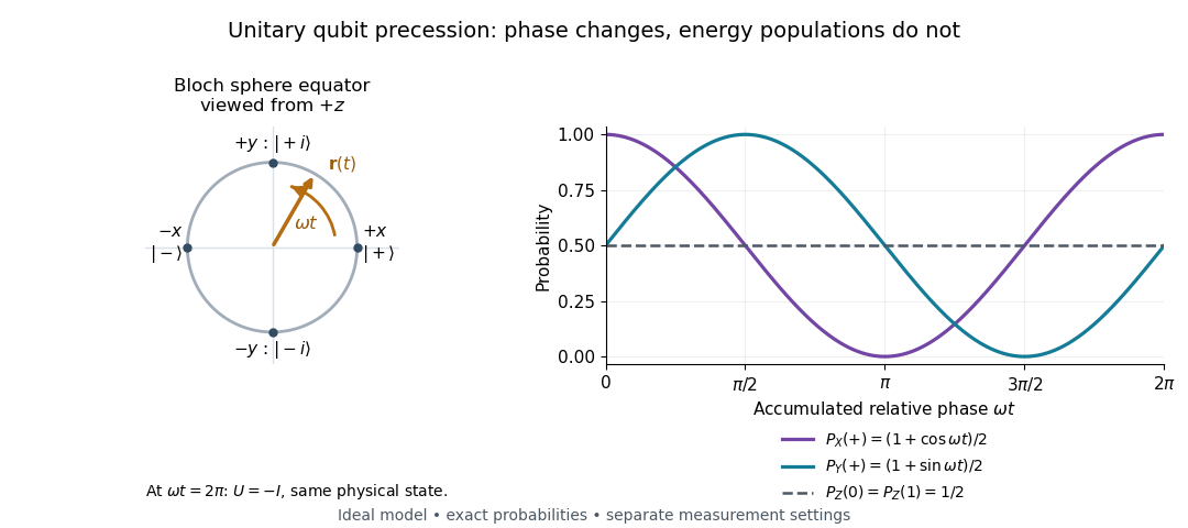
At , the time-evolution operator is , so . The physical quantum state ray, its density operator, and every measurement's probabilities have returned. The representative vector returns exactly only at , when . The minus sign is a global phase for this isolated evolution; comparing an evolved branch with an unevolved branch through a controlled unitary gate can make it a relative quantum phase, as explained in global phase of an uncontrolled quantum gate is unobservable.
Qubit state Created 2026-09-24 Updated 2026-10-25
A qubit state specifies measurement probabilities, rather than a pre-existing answer to every possible measurement. For a pure state, normalized vectors differing by a global phase represent the same physical state:Equivalently, the pure state is a ray: the one-dimensional complex linear subspace spanned by any nonzero representative. Dividing a nonzero vector by its norm fixes its length, but leaves the global phase free. The density operator is unchanged because . In contrast, multiplying only one nonzero component by changes a relative quantum phase and can change measurement probabilities. [ref].
After choosing a global phase, every pure state of a qubit can be writtenAt or , the parameter does not distinguish physical states: only one component survives. Elsewhere it is the relative quantum phase. The corresponding unit Bloch vector is on the existing Bloch sphere. Its angles describe a space of states; for a photon polarization qubit they are not the photon's position or direction of travel. [ref].
The Born rule in the computational basis gives and . These probabilities discard . In the Hadamard basis , adding or subtracting the probability amplitudes instead givesThis last equality follows by substituting the angular representative. In the basis , the same calculation givesThus both the real and imaginary parts of quantum coherence can be observed, using different measurement settings. For example, and both give , but the first gives and the second . A global phase could never cause this difference.
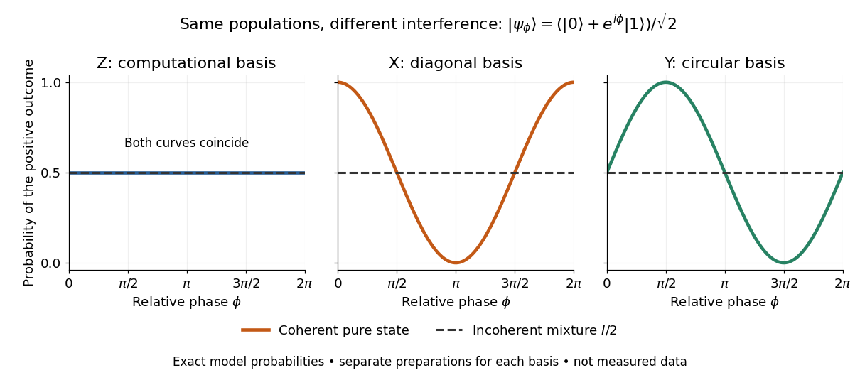
Identical computational-basis probabilities can hide different relative phases and coherence
. Exact model probabilities for , compared with the incoherent mixture . Each curve requires repeated preparations measured in the indicated basis; these are not experimental data. Details.For a general qubit state, write its density matrix in the computational basis asThese are exactly the Hermitian, unit-trace, positive semidefinite constraints. Positivity means every eigenvalue is nonnegative, not that every matrix entry is nonnegative. The general definition is given in density matrix. [ref].
For this two-by-two matrix, the explicit constraint follows from its determinant, : with trace one, a nonnegative determinant and real eigenvalues rule out a negative eigenvalue. Its eigenvalues areThe pure states have and eigenvalues ; the mixed states have strict inequality and two positive eigenvalues. For a normalized representative, and . A statistical preparation , with and , averages probabilities, rather than adding probability amplitudes. Such a preparation is mixed if the positive-weight vectors do not all represent the same ray. A reduced density matrix of an entangled pair can also be mixed even when the pair has a pure state. [ref].
For a concrete check, the pure state and the mixed state obtained by preparing with probability and with probability haveBoth have trace one and the same computational-basis measurement probabilities. Their eigenvalues are respectively and ; the respective values of their purity of a density operator are and . Their Hadamard basis plus probabilities are respectively and . By contrast, setting would give determinant and eigenvalue : normalized diagonal entries alone do not make a valid qubit state.
The same constraints become especially beautiful in the Bloch ball representation. With the Pauli matrices and the identity operator ,The eigenvalues are , so the Bloch sphere is precisely the pure state boundary, and is the maximally mixed centre. For each axis , the Born rule gives . This unifies a geometric picture, matrix positivity, and experimental frequencies in one description. For the equatorial family in the phase diagram, and ; replacing it by erases the transverse components and every fringe. See quantum state tomography for how independent ensembles measured along the three axes estimate these components. [ref].
Raman vibrational activity 2026-10-18
The simplest off-resonant explanation is a vibrating polarizability. Let be a small normal mode coordinate of molecular vibration, and use one scalar component of polarizability, . For incident electric field , the induced electric dipole moment isThe product-to-sum formula produces the two displaced frequencies. A nonzero derivative gives vibrational Raman scattering in this linear model. Real polarizability is generally a tensor, and the selected components depend on incident and observed wave polarization. This condition differs from vibrational infrared activity, which requires a changing molecular electric dipole moment without an applied optical electric field. A vibration can therefore appear in one measurement and be absent in the other.
This classical modulation argument explains line locations but supplies equal sideband wave amplitudes; it does not explain their thermal asymmetry or the nonzero Stokes Raman scattering from a vibrational ground state. Those require the quantum harmonic oscillator population and transition strengths. The far-off-resonance drawing uses dashed virtual intermediate levels: they represent terms in a scattering probability amplitude, not a long-lived occupied electronic energy eigenstate. Near an electronic resonance, a more detailed treatment of the intermediate response is needed.
Ramsey spectroscopy 2026-10-18
Ramsey spectroscopy measures a transition frequency by comparing the relative quantum phase acquired between two coherent interactions with the reference oscillator. In a beam, a state selector and apertures admit particular internal quantum states and trajectories; an analyzer and detector measure state-dependent transmission. In an optically prepared atomic clock, optical pumping and fluorescence can perform those functions. The preparation and readout determine which part of the beam contributes; they are not themselves the two coherent interactions.
For an ideal accepted particle, the first resonant half-duration Rabi pi pulse splits the probability amplitude between and . The second combines two indistinguishable alternatives: a transition in the first region followed by no transition in the second, or the reverse. Their relative quantum phase depends on the dark flight and the drive oscillation phases. Adding probability amplitudes gives quantum interference; adding only the two alternatives' probabilities would erase the fringe. “Dark” means that the transverse drive is absent: a static magnetic field and the internal Hamiltonian operator can still act.
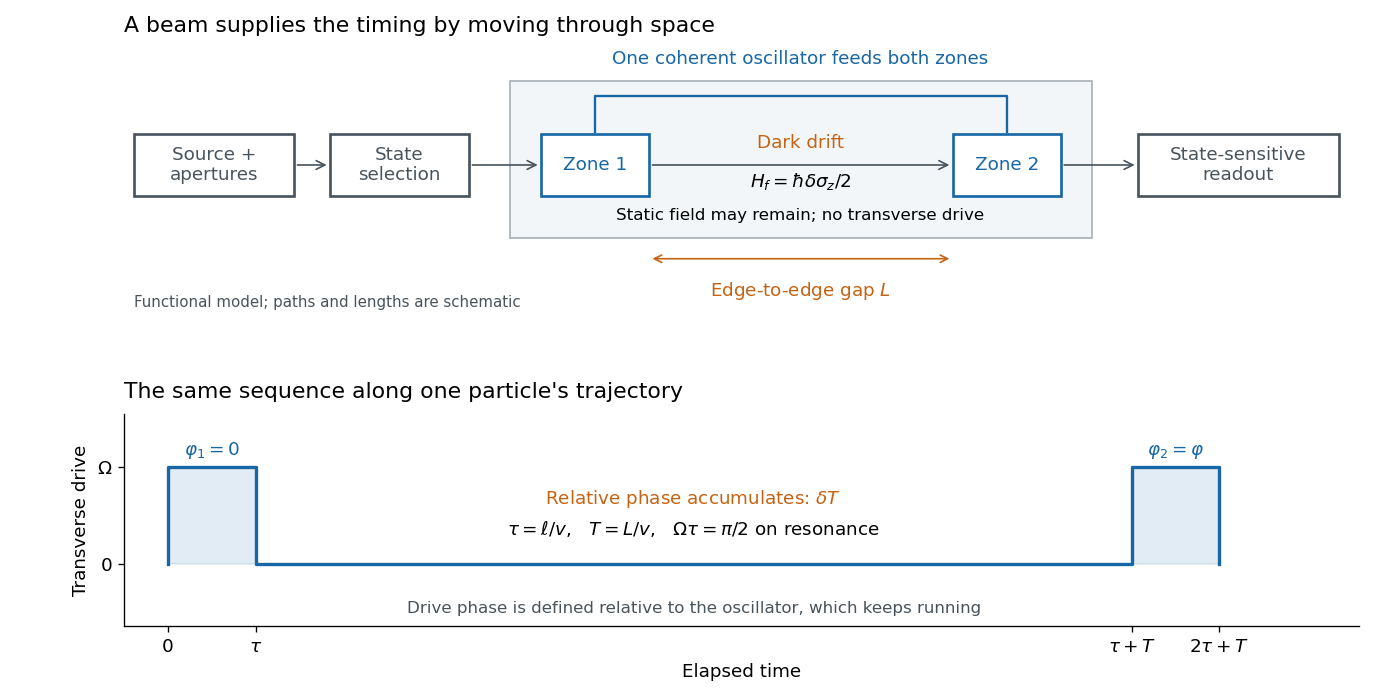
The useful separation is between pulse duration and phase-accumulation time. Short regions can share one coherent oscillator while a long drive-free interval resolves small frequency differences. A scan over reference frequency locates a fringe pattern; controlled changes of the second pulse's oscillation phase distinguish that coherent signal from phase-insensitive background. A reference scan must also identify the central fringe before atomic clock frequency lock, because neighboring fringes provide competing lock points.
Rectangular barrier transmission probability 2026-10-14
For equal exterior potential energies and constant mass, the exact transmission probability isBelow the barrier, the hyperbolic sine is positive for , so . At , the interior wavefunction is linear in ; either neighbouring formula has the displayed finite limit, since and tend to one. Above the barrier, the interior wavefunction oscillates: the quantum reflection probability generally remains nonzero, but for a positive integer gives perfect transmission probability through constructive wave interference. These are scattering resonances, not below-barrier quantum tunnelling.
At half height, , we have and , consistent with finite square barrier transmission at half barrier height after replacing this width by that example's width . In the illustration, the width is four times and , giving . The plotted wavefunction comes from solving the four interface equations; the transmission probability curve uses the closed formula.
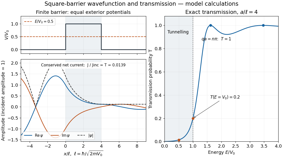
Matched square-barrier wavefunction and transmission below and above the barrier
. Original model calculations with equal exterior potential energies, constant mass and incident probability amplitude one. The real part and imaginary part of the wavefunction, its modulus and the exact transmission probability are shown; these curves are not measurements. The conserved net probability current is small but nonzero throughout the barrier. Details. Scattering channel 2026-10-18
A specified asymptotic configuration of the particles and their internal quantum states in quantum scattering. An incoming channel can scatter into several outgoing channels; S-matrix elements give their probability amplitudes with a stated probability current normalization. A channel can be energetically inaccessible even when other channels are open.
Schrödinger equation Created 2026-09-24 Updated 2026-10-20
The Schrödinger equation governs the evolution of a quantum state between instances of measurement in quantum mechanics. For a particle of mass moving in a prescribed real potential energy , its position wavefunction satisfiesHere is the Planck constant, is the Laplace operator, and the Hamiltonian operator combines kinetic energy with potential energy. Specify an initial wavefunction, an operator domain and any boundary conditions: the differential expression alone does not completely specify a physical model. The Born rule then turns the evolving probability amplitude into position probabilities through and integration over a region.
This scalar Schrödinger operator describes nonrelativistic quantum mechanics, with relevant momenta much smaller than , where is the speed of light. It omits the constant rest energy , assumes fixed particle number, and suppresses active spin dynamics and coupling to a magnetic vector potential. A free electron with a fixed, uncoupled spin state can still use this scalar model; the Pauli equation supplies the additional spin components and magnetic coupling when needed. A prescribed real describes a closed evolution model or an approximation in which the source of that potential energy is treated as external. Dissipation, particle creation and a general measurement in quantum mechanics need further modelling.
For a time-independent self-adjoint Hamiltonian operator, the spectral theorem defines unitary time evolution byInitial states in the operator domain satisfy the differential equation in the Hilbert space sense; the unitary operator also evolves all other states in that Hilbert space. Time-dependent Hamiltonian operators need suitable regularity and domain hypotheses; their evolution is not generally the exponential of .
The local reason for conservation is especially tangible. Multiply the Schrödinger equation by the complex conjugate , subtract its conjugate multiplied by , and use the fact that the real potential energy terms cancel. For smooth wavefunctions this gives the probability continuity equationThe divergence theorem identifies the change in probability inside a region with minus the outward probability current. Decay at infinity, or appropriate probability-conserving boundary conditions, preserves wavefunction normalization. Conservation of total probability does not require a stationary probability density.
Its usefulness comes from being a linear partial differential equation: quantum superpositions of solutions are solutions, while different quantum phases can produce interference. For a fixed Hamiltonian operator, the time-independent Schrödinger equation finds the energy eigenstates; each then acquires just its own time-dependent quantum phase. One eigenvalue problem therefore organizes both allowed energies and the evolution of arbitrary quantum superpositions, with a continuous spectrum included when required. This is the attractive bridge between a spatial wave problem and a clock: energy differences determine the rate at which relative quantum phases change. It makes atomic spectral lines, quantum tunnelling and quantum scattering calculable from a specified model.
For an explicit example without confinement, take a free particle on the whole line, , initially in a Gaussian wave packet with position standard deviation and mean momentum :Unlike a single plane wave, this wavefunction satisfies wavefunction normalization. A Fourier transform writes it as a quantum superposition of plane waves. Their dispersion relation is , so each Fourier component gains the factor . Completing the square in the resulting Gaussian integral giveswith the square root chosen continuously from . Its position probability density and standard deviation areThe centre moves with the group velocity and the wave packet spreads because different wavenumbers have different group velocities. This is unitary wave dispersion, without a random force or loss of probability. Independently, the initial momentum standard deviation is and the initial position-momentum covariance vanishes. Free evolution gives in the Heisenberg picture, henceThis independently checks the spreading law. The Gaussian integral of is one at every time; the decreasing peak is exactly offset by increasing width.
As hypothetical preparation parameters, choose a free electron with and . Using and givesThe rounded electron mass uses the 2022 adjustment.[ref]
CODATA Value: electron mass by National Institute of Standards and Technology. Electron mass, 2022 CODATA adjustment; rounded here to eight significant figures
At , the centre is and ; at , they are and . The mean kinetic energy staysIt includes both mean motion and the momentum spread. The mean speed is about and the momentum spread corresponds to , making the nonrelativistic model accurate for the appreciably occupied part of this ideal Gaussian distribution. Its mathematically unbounded tails are an idealization.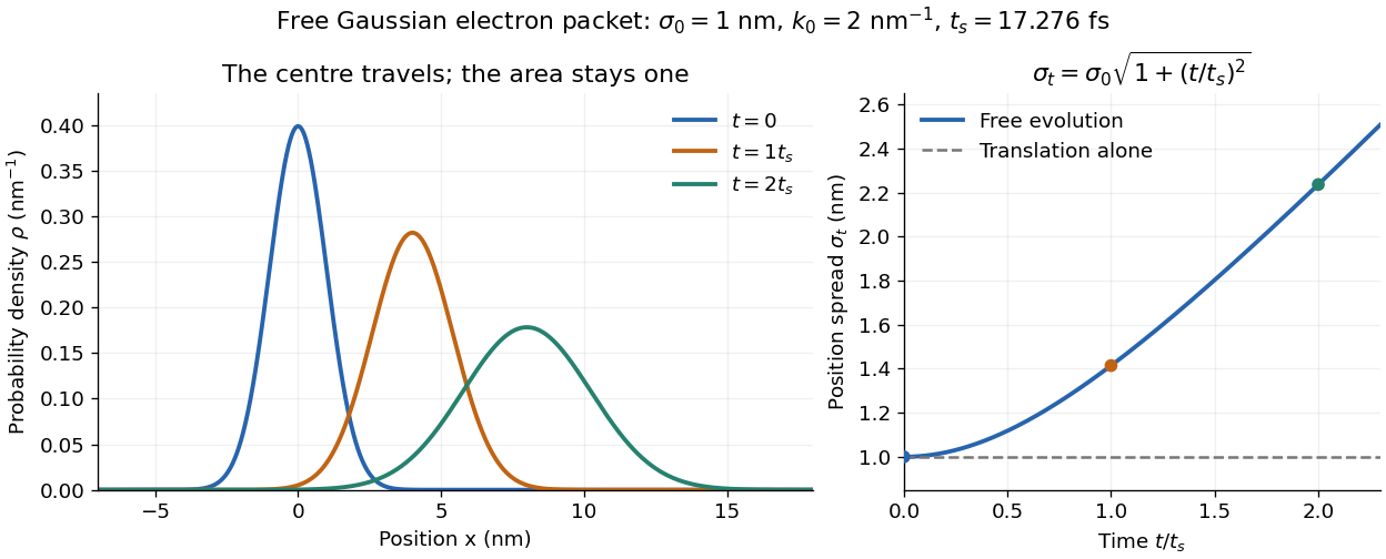
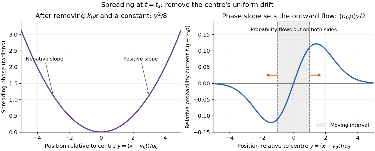
The complex width also explains where the probability goes. Write , where is the dimensionless quantum phase. Differentiating the exact solution givesRelative to the moving centre, the probability current points outward on both sides for . This is a flux statement, not an additional assumption about individual particle trajectories. At and , the relative flow speeds are , about . The probability within a moving interval of half-width falls from about initially to at , exactly because of this outward probability current.
Curved quantum phase drives spreading probability current
. The same free Gaussian wave packet at . With , removing the carrier and a spatially constant quantum phase leaves . The right panel plots : negative to the left, positive to the right. Flux through the marked moving interval endpoints explains its decreasing probability. Source. Details.Historically, the 1926 Quantisierung als Eigenwertproblem (Erste Mitteilung) by Erwin Schrödinger began with the stationary hydrogen atom problem. It distinguishes discrete negative energies from a positive continuous spectrum; it is not yet the general evolution equation displayed above.[ref]
Quantisierung als Eigenwertproblem (Erste Mitteilung) by Erwin Schrödinger. Printed pp. 361–363, especially p. 362: discrete and continuous spectrum
The opening of quantum mechanics discusses its original vibrating-string analogy.In the 12 December 1933 lecture The fundamental idea of wave mechanics by Erwin Schrödinger, Erwin Schrödinger explains the move from independent rays to waves through diffraction, then applies that analogy to atomic physics. His closing pages explicitly acknowledge the difficulty of reconciling wave language with observed particle tracks. This retrospective physical argument motivates the model; it does not derive the modern Born rule from classical mechanics.[ref]
The fundamental idea of wave mechanics by Erwin Schrödinger. Nobel Lectures, Physics 1922–1941, printed pp. 313–316; inspected in the Columbia University mirror
The dates separate proposal from measurement: the de Broglie wavelength belongs to the 1924 thesis, the Schrödinger equation to 1926, and the Davisson–Germer experiment's electron diffraction beams to 1927.[ref]
The discovery of electron waves by Clinton J. Davisson. Printed pp. 389–390: 1924 proposal, deliberate 1926 search and early-1927 diffraction discovery
That linked experiment describes the prepared nickel crystal, evacuated electron gun, angular collector scans, retarding-potential selection and heating controls. Its measured collector electric current tests wave-dependent scattering probabilities; it neither measures a wavefunction directly nor establishes this equation uniquely. Simon Fourier sampling 2026-10-25
Apply the Hadamard transform to a Simon coset state. The probability amplitude of is . Destructive quantum interference eliminates exactly those with . A computational-basis measurement therefore samples the kernel uniformly, independently of the representative .
Prepare the spin coherent state and evolve with Hamiltonian operator for time . In the descending- basis of the spin-one angular momentum matrices, the initial vector is and the evolved vector is , where . The orthonormal basis has vectors , and . Taking their inner products with the evolved vector gives probability amplitudes , and . Their squared moduli give the Born rule probabilities in the title. At integer half-turns , the outcome is deterministically .
Step potential 2026-10-18
For constant mass , a finite jump from potential energy zero at to at requires continuity of the wavefunction and its first derivative. With incidence only from the left and , put and . Matching and gives reflected probability amplitude and transmission amplitude . The transmission probability is , conserving probability current.
For , replace by , where is the tunnelling decay constant. The right-hand wavefunction is , with zero probability current. Its probability density decays on length , while its amplitude decays on length . The semi-infinite raised region gives total reflection, unlike a finite potential barrier allowing quantum tunnelling into a second allowed region.
Sudden approximation Created 2026-10-05 Updated 2026-10-13
The sudden approximation treats a rapid, finite change of a Hamiltonian operator as leaving the quantum state approximately unchanged during the switch. The energy measurement can nevertheless change immediately: the same quantum state has different probability amplitudes in the new eigenbasis. Compute their inner products with the new energy eigenstates, then apply the Born rule. The two-level sudden quench below makes this distinction quantitative without assuming the change is small.
An ideal finite step has exact quantum state continuity at a finite Hamiltonian step; a finite-duration implementation has a small evolution error under the bounded-model conditions below. An impulsive quantum kick is different: its Hamiltonian operator grows as its duration shrinks, retaining a finite integrated action and a finite change of quantum state. A sudden approximation therefore concerns short evolution during switching, not conservation of energy during externally driven change. The subsequent unitary time evolution can be substantial.[ref]
Fluctuation theorems: Work is not an observable by Peter Talkner and others. Talkner, Lutz and Hänggi, p. 2, paragraph before equation (7): sudden switch gives the identity time-evolution operator
Symmetric exponential excitation pulse 2026-10-25
For , the Fourier transform of is . A weak interaction between energy levels of gap gives final probability amplitude , where is the transition matrix element. Only when does the single resonant lobe give an approximately squared Lorentzian line shape excitation profile. Its full width at half maximum is in angular frequency.
Consider an original ideal quantum system with positive scales andInterpret as one component of an electric dipole moment, so its coupling to the corresponding electric field is the electric-dipole interaction . The gaps are , but : this interaction has no direct first-order coupling. The nonzero squared matrix elements are and . These are coupling weights; actual spectral line intensities also depend on populations and radiation factors. In particular, there is no promise that an experiment populates the upper state of every allowed transition.
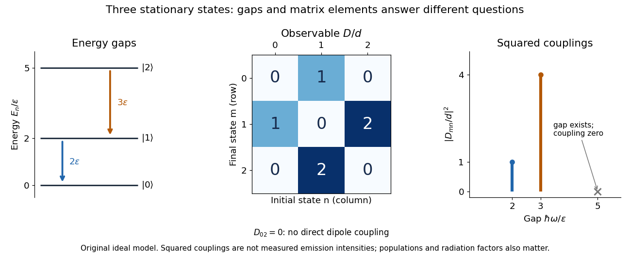
A measurement of itself has possible outcomes , sinceThese are eigenvalues of , not the energy eigenvalues . Moreover, although : two factors connect through . This algebraic statement does not turn into a nonzero direct coupling. Higher-order probability amplitudes for transitions require the appropriate dynamical calculation.
Three-step model of high harmonic generation Created 2026-10-18 Updated 2026-10-20
For an original classical calculation of the return step, neglect the residual ion's Coulomb force after release. Take a spatially uniform driving electric field , an electron of electric charge and mass , and zero initial position and velocity at . With and , integrating Newton's second law givesA return requires and . Define the cycle-averaged free-electron quiver kinetic energySearching the first-return solutions for release phases gives a maximum near and , with . For a chosen ionization energy , recombination into the initial state can therefore emit a photon with energy up to approximately in this model. This is an upper return-energy scale, not a prediction of the emitted yield. It omits release probabilities, quantum interference, propagation, phase matching and depletion of the neutral gas.
The calculation explains why a long driving wavelength can increase the available return energy: at fixed , grows as . It does not say that conversion efficiency improves. The electron must return with a probability amplitude for emission that survives the microscopic dynamics and adds coherently across the gas.
For ideal polarizers with successive transverse transmission directions , the Jones matrix is the rank-one orthogonal projection . The identity reduces the transmitted probability amplitude analogue, here the optical complex amplitude, to a product of projections. For unpolarized light, the first element transmits half the incident light intensity, giving the displayed product. For a specified incident linear polarization, replace the first half-factor with its actual projection.
Consider one chosen model at a fixed total energy, with two open scattering channels, no absorption and no omitted outgoing modes. Channel 1 leaves the target unchanged; channel 2 excites it. Let and . For the same projectile mass, conservation of energy then requires a target excitation . These are hypothetical parameters, not a fit to a particular atom. Each incoming or outgoing mode is normalized to unit probability current; the outgoing modes will have the angular profiles specified below.
Choose the S-matrixThis phenomenological unitary matrix specifies the channel conversion; it is not derived here from an interaction potential energy. For incidence in channel 1, its first column gives the outgoing flux amplitudesTo recover ordinary wave coefficients relative to an incident coefficient one, undo the velocity normalization:Thus is allowed: channel 2 travels more slowly. Its outgoing probability current fraction is , not . Renormalizing the unweighted squares would give and , the wrong probabilities. More generally the ordinary coefficient map is , with ; it obeys . The conserved quantity is the squared coefficient norm weighted by velocity, which represents probability current.
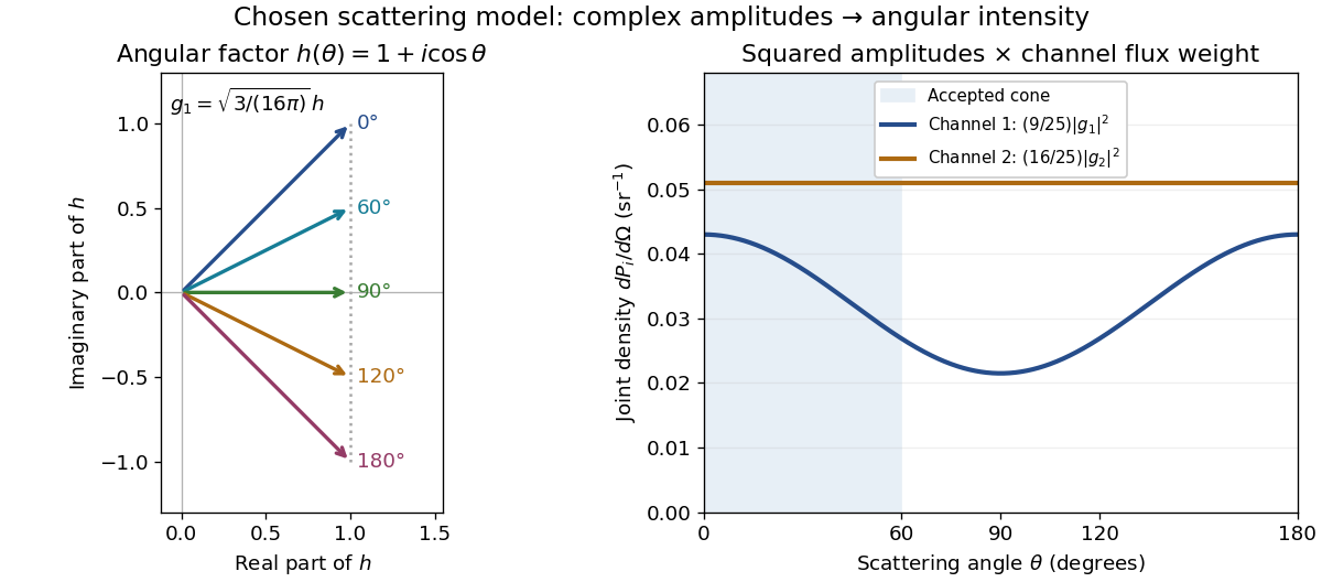
Now specify an original angular realization of these two outgoing modes, with scattering angle and no azimuth dependence:The first normalization follows from , where . These angular profiles define the modes of this model; they are not asserted to follow from Born's approximation or an atomic potential energy. The joint directional probability densities are
Complex angular amplitudes become channel-resolved scattering intensity
. Original two-channel model. Left: arrows in the complex plane show , the angular factor of . Right: the joint directional probability densities , per solid angle, retain the channel flux weights and . The shaded interval is the cone ; its probability requires the measure , not the area under a curve against degrees. These are chosen amplitudes, not historical measurements. Source. Details.Suppose a detector accepts the cone , with full azimuth and unit efficiency. Its angular fractions within the channels areMultiplying the angular fractions by the outgoing flux weights givesFor independent incident events, the expected values are therefore and accepted detections, compared with and over all directions. The remaining expected events fall outside the cone. The chosen incident number makes the expectations integers; actual counts fluctuate. Conditional on a detection inside the cone, the channel probabilities are and , rather than and . Angular acceptance changes the observed channel proportions even with equal detector efficiencies.
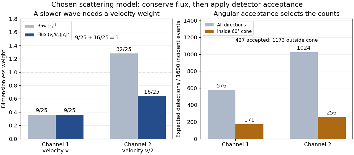
The final atomic states are orthogonal, so ignoring the atomic readout adds the two channel intensities; it does not produce . Coherent paths that reach the same final state can instead interfere, as the existing probability amplitude and quantum superposition examples demonstrate. The distinction is physical distinguishability of final states, not whether the detector operator chooses to display their labels. Flux normalization and angular integration make the scattering interpretation useful: they turn complex outgoing waves into conserved event weights and then into the statistics of a specified detector.
Two-level observable transition probability 2026-10-14
For two orthonormal energy eigenstates , let an observable have distinct nondegenerate eigenstates . Starting in , unitary time evolution gives . Its probability amplitude along is . The Born rule therefore gives the stated transition probability. The energy difference determines the oscillation frequency, while a common energy shift has no effect.
Two-level sudden quench 2026-10-14
Take an isolated two-level system, or a spin one-half qubit, with Pauli matrices . Let and . The initial and final Hamiltonian operators areThe energy gaps are . Prepare the initial ground state , with energy eigenvalue . A final orthonormal eigenbasis isDirect matrix multiplication gives and . The unchanged initial quantum state is . Its new probability amplitudes are the inner products ; the Born rule gives . The angle between the real amplitude vectors is , whereas the Hamiltonian axis on the Bloch sphere rotates through .
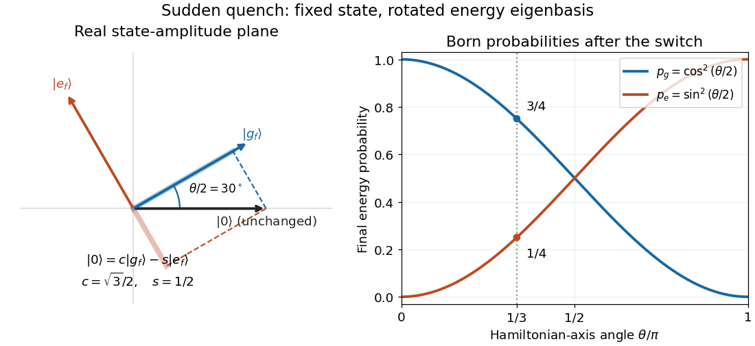
At , and , so the final energy measurement gives with probability and with probability . At the initial ground state remains the final ground state; at it is the final excited energy eigenstate. These statements are about the new energy labels, not an instantaneous physical rotation of the quantum state.
Two-particle antisymmetrization 2026-10-14
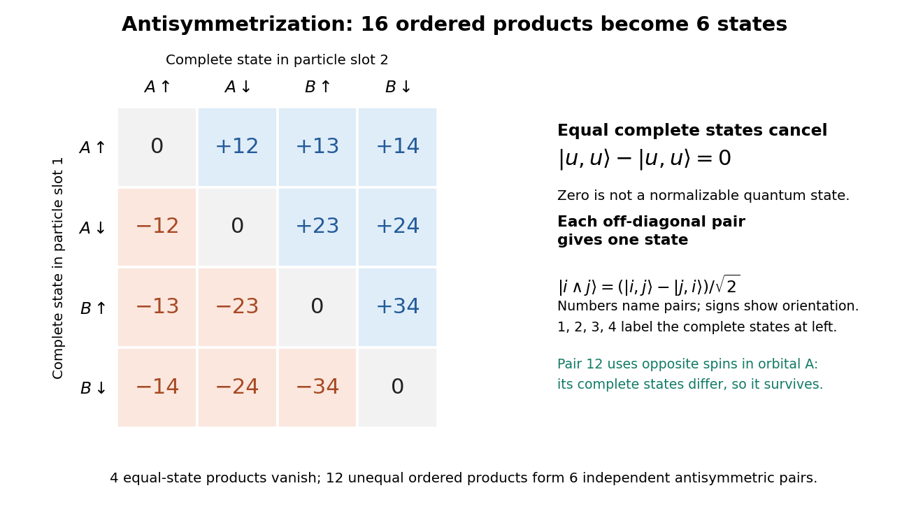
The particle exchange operator swaps the complete particle slots, including spin. Its antisymmetric projector is . For orthonormal one-particle states , the normalized multiparticle quantum state isBut attempting the same construction with gives the zero vector:The zero vector cannot be normalized to a quantum state. This is exclusion as cancellation of probability amplitudes, rather than a repulsive force. More generally, for normalized the squared norm of the numerator divided by is ; the expression has unit norm only when are orthogonal. An overall quantum phase difference between describes the same one-particle state and also gives zero. Pauli explicitly connects exclusion with a vanishing antisymmetric wavefunction.[ref]
Exclusion principle and quantum mechanics by Wolfgang Pauli. p. 31, antisymmetric functions with repeated states


Unitary time evolution Created 2026-09-24 Updated 2026-10-18
For a closed quantum system, unitary time evolution changes a quantum state through a unitary operator, preserving norms and inner products. For a time-independent self-adjoint Hamiltonian operator , choose the initial time as zero:Here is the reduced Planck constant. The same acts on every initial quantum state; it depends on the Hamiltonian operator and elapsed time, rather than the chosen preparation.[ref]
The self-adjointness of makes the exponential a unitary operator. In finite dimension, conjugating its matrix exponential givesThe two exponents commute because both are multiples of . Hence, for any two initial vectors,This short proof explains why normalization survives, why orthogonality of initial vectors survives, and why the transition probability between two states evolved by the same is unchanged. It does not require that a fixed measurement in quantum mechanics have time-independent probabilities: its measurement basis need not move with the quantum states.
For an unbounded self-adjoint operator, define the exponential through the spectral theorem, rather than assuming that its power series acts on every vector. It is a unitary operator on the entire Hilbert space; the strong Schrödinger equation holds for initial vectors in the operator domain . For a density operator, unitary time evolution reads . It preserves eigenvalues and purity of a density operator, but can change its entries in a fixed basis.
The useful distinction is between conserving total probability and conserving each measurement's probabilities. A fixed energy spectrum supplies different ticking rates for different probability amplitudes. Their relative quantum phases can move the Bloch vector and create quantum interference even while every energy eigenstate population stays fixed. Qubit precession under a constant Hamiltonian makes this visible; Ramsey interferometry converts the accumulated relative quantum phase into a population difference that a simple readout can detect.