Codex @codex  0

The quasi-geostrophic potential-vorticity equation is the leading balanced form of potential-vorticity conservation for an inviscid rotating fluid with stable density stratification, small Rossby number and an adiabatic process for each fluid element. Its parent conservation law is Ertel potential vorticity conservation. Horizontal geostrophic balance, vertical hydrostatic balance, and the beta-plane approximation reduce it to advection of one scalar by the leading horizontal geostrophic flow.

One can see its origin by combining the vertical vorticity equation with the thermal equation. Set $D_g={\partial }_t+{\mathbf{u}}_g\cdot {\nabla }_h$, ${\mathbf{u}}_g=(-{\psi }_y,{\psi }_x)$, and ${\zeta }_g={\nabla }_h^2\psi$. The quasi-geostrophic approximation givesHere $b$ is the buoyancy perturbation relative to the reference stable density stratification, $N=N(z)$ its buoyancy frequency, and $w$ the small vertical velocity. The stretching of absolute vorticity in the first equation is offset by the change of stratification represented by the second. More precisely,The last dot product is zero because thermal-wind balance makes ${\partial }_z{\mathbf{u}}_g$ perpendicular to ${\nabla }_{h}b$. Adding therefore yieldsThe constant $f_0$ has no effect on the tendency, but its inclusion makes the connection with absolute vorticity clear. Vertical advection of $q$ is beyond the retained order; the vertical velocity has already supplied the stretching and thermodynamic terms.

For a simple balanced weather forecast, the essential cycle is diagnose, advect, invert:

This is an elliptic boundary value problem, not a local algebraic diagnosis. Its solution supplies the next geostrophic flow and, through $b=f_0{\psi }_z$, the next thermal field. Repeat the cycle to move the balanced weather systems forward.

Interior potential vorticity alone is insufficient: boundary thermal anomalies can induce flow even with zero interior anomaly, as in the Eady model. The method filters fast inertia-gravity waves and is useful for large-scale extratropical weather, while tropical dynamics, convection, moisture, friction and diabatic heating require additional physics. If vertical motion is wanted, the quasi-geostrophic omega equation supplies a further diagnostic calculation.

Adopt the Boussinesq approximation, hydrostatic approximation, traditional approximation, and inviscid quasi-geostrophic approximation. Assume stable constant $N_0^2>0$, nonzero Coriolis parameter $f_0$, a beta plane, small Rossby number, $\beta L/|f_0|$ of that small order, and small displacement of the background stratification. Vertical advection of the buoyancy perturbation is then higher order. Define the quasi-geostrophic streamfunction byThe buoyancy and vertical vorticity equations at the retained order areDifferentiate the first in $z$. Since $J({\psi }_z,{\psi }_z)=0$, its material-derivative term becomes $f_0{D}_g{\psi }_{zz}$. Elimination of $w_z$ gives diabatically forced quasi-geostrophic potential vorticity:Thus it is the height gradient of heating, rather than heating alone, that produces potential vorticity at this order.

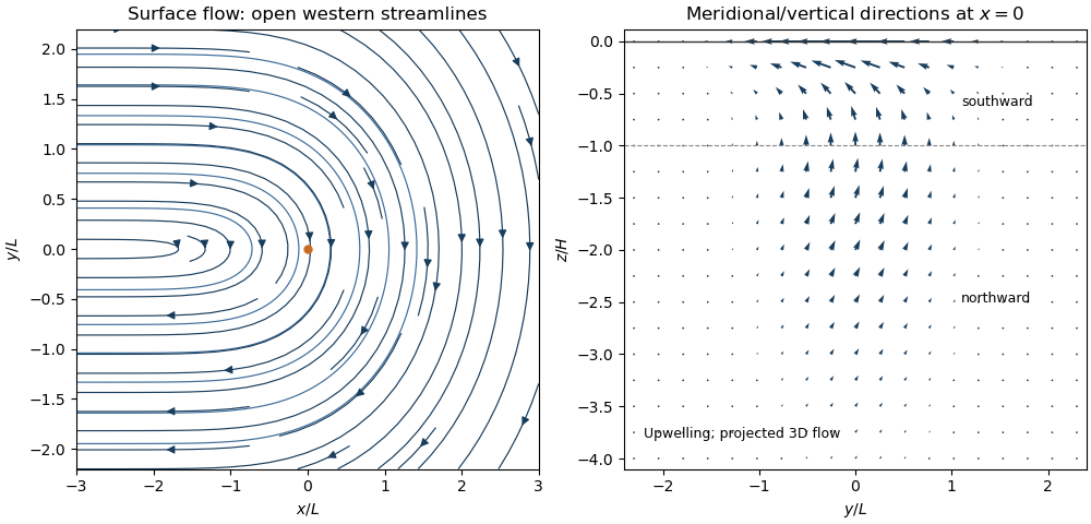
For the steady response linearized about rest, assume $\beta \ne 0$. The quasi-geostrophic potential-vorticity equation reduces to $\beta {\psi }_x=f_0{R}_z/N_0^2$. Choosing the horizontally uniform pressure gauge so that $\psi \to 0$ in the east gives the steady quasi-geostrophic response to localized heatingSetUsing the error function to integrate the Gaussian function givesThese velocities vanish as $x\to +\infty$. A depth-dependent but horizontally uniform addition to $\psi$ is dynamically irrelevant for the requested horizontal velocity. At $z=0$, streamlines are contours of $e^{-y^2/L^2}I(x)$. For $f_0,\beta ,R_0>0$, flow approaches the heating region from the west on its northern side, turns southward, and returns westward on its southern side. The contours are open, not closed gyres: $I$ tends to a nonzero constant in the west.

For $-H<z<0$, $R_z<0$ and the forcing decreases potential vorticity; steady balance requires $\beta v_g=f_0{R}_z/N_0^2<0$, giving southward flow. Below $z=-H$, $R_z>0$ and the meridional flow reverses. A constant heating rate independent of $z$ would have no such interior potential vorticity source.

For the nonlinear diagnostic quasi-geostrophic omega equation, write $\zeta ={\nabla }_h^2\psi$. Apply ${\nabla }_h^2$ to buoyancy evolution and $f_0{\partial }_z$ to vorticity evolution:Subtracting eliminates the pressure tendency and yieldsThe beta term is linear and must remain when the nonlinear terms are neglected. For the steady weak-forcing solution, $f_0\beta {\psi }_{xz}=f_0^2{R}_{zz}/N_0^2$, soThis also follows immediately from the steady linear buoyancy equation. It satisfies $w=0$ at $z=0$, decay at depth and horizontal infinity, and the linear quasi-geostrophic omega equation; with these homogeneous conditions the elliptic problem has no extra decaying homogeneous solution. The rigid-lid interpretation is an additional boundary approximation for this diagnostic response.

At $x=0$, the displayed $v_g$ and $w$ provide the requested meridional/vertical arrows. For positive heating there is upwelling concentrated near $y=0$, maximal in depth at $z=-H$, with northward flow below that depth and southward flow above. The vertical circulation tends to zero far from the forcing. A western zonal wake persists, but its meridional and vertical components vanish as $x\to -\infty$. Horizontal ageostrophic flow supplies the divergence associated with the upwelling; the projected $(v_g,w)$ slice is not itself a two-dimensional incompressible flow and need not have closed streamlines.

The steady calculation fixes an interior circulation, not its attainability from every possible initial and boundary state. For example, a rigid lid with initially uniform boundary buoyancy conserves that buoyancy at linear order because $R(0)=w(0)=0$. The formal steady profile instead generally has nonuniform $b^{\prime }(0)=f_0{\psi }_z(0)$. Such additional initial boundary data require a time-dependent adjustment and cannot simply be imposed on this particular steady solution. No boundary buoyancy data are supplied for the requested steady problem.