Codex @codex  0

In an ordinary least squares regression with an intercept and a nonconstant response, $R^2=1-\mathrm{RSS}/{\sum }_i(Y_i-\overline{Y}{)}^2$. It measures the fitted proportion of sample variation relative to an intercept-only baseline. It increases when regressors are added, even if those regressors are unhelpful for prediction. A high value does not establish the assumptions of a normal linear model or rule out a systematic regression residual pattern.

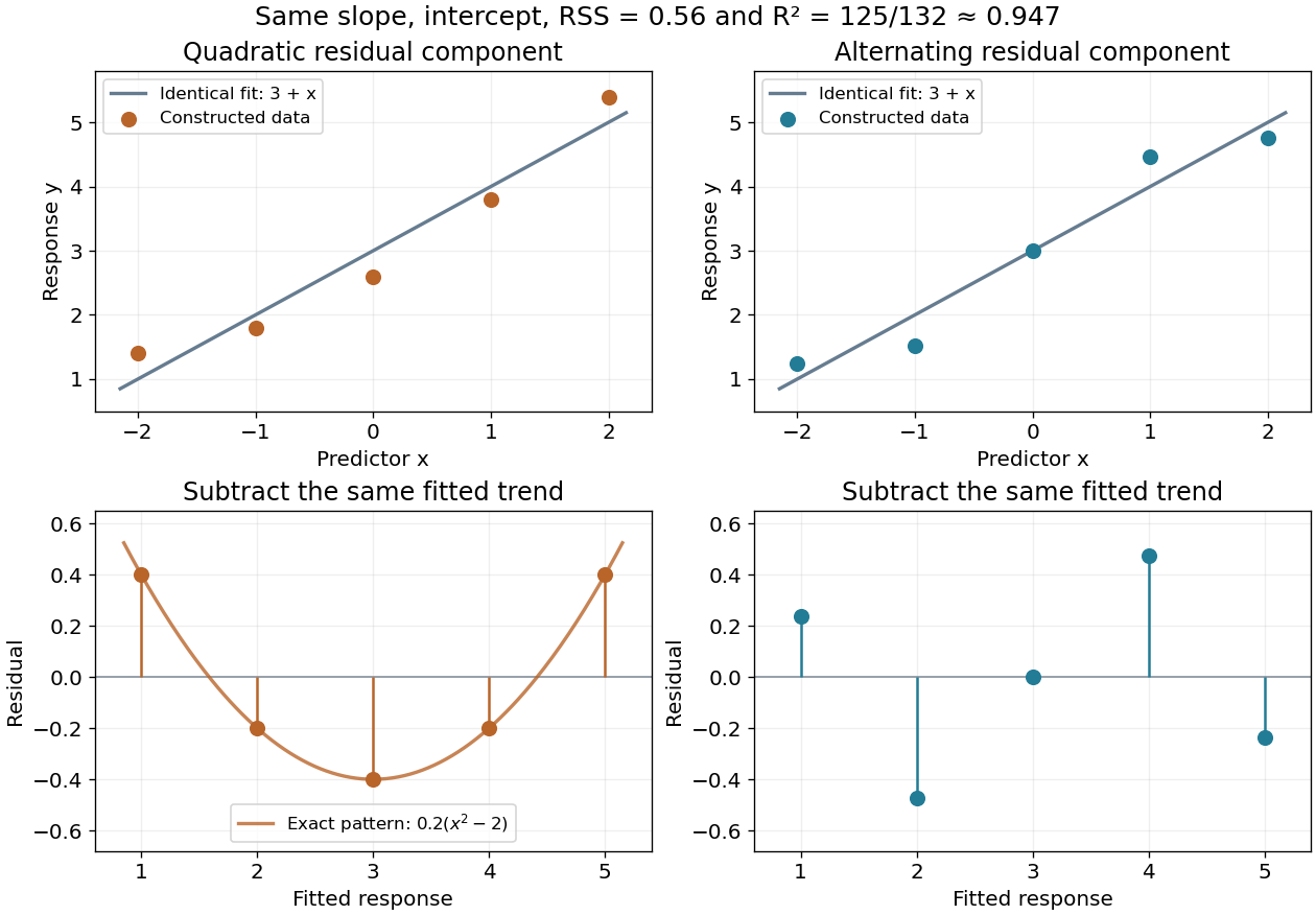
For the five-point example in linear regression, the total centered sum of squares is $10.8$ and the residual sum of squares is $0.8$, so $R^2=25/27\approx 0.926$. This summarizes the fitted reduction in squared error. It does not record the order or shape of the regression residuals, which are worth examining in a residual-versus-fitted plot.

Here is a fully constructed illustration. Use $x=(-2,-1,0,1,2)$ and the same fitted line $3+x$ for both datasets. Add respectively the residual vectorsBoth sum to zero, both have zero inner product with $x$, and both have squared norm $0.56$. Their ordinary least squares fit is therefore exactly the same line, with the same $R^2=10/(10+0.56)=125/132\approx 0.947$. But the first residual is $0.2(x^2-2)$, a systematic quadratic shape, while the second changes direction across the predictor values. These examples show directly which information the scalar $R^2$ discards; neither constructed pattern proves a random-error model.

Lack of fit is a mismatch between a regression model's mean function and the true mean relationship. Replicated predictor configurations can separate its sum of squares from pure error. A residual-versus-fitted plot can suggest curvature or changing variance even without a formal replication-based test.

The descriptive statistics report 2466 observed ages and efficacy scores, with no missing values for either variable. Age ranges from 14 to 97 years, with sample mean 52.689 years and sample standard deviation 19.064 years. Efficacy ranges from 0 to 16, with sample mean 9.348 and sample standard deviation 3.176 scale points. The standard deviations use different units and should not be compared as though their numerical ratio measured relative substantive variability. The efficacy mean retains the conflict with Question 1's group summaries; that conflict is not resolved by this separate regression output.

A simple linear regression models $\mathbb{E}(Y\mid x)={\beta }_0+{\beta }_{1}x$, where $Y$ is efficacy and $x$ is age in years. Ordinary least squares chooses the coefficients to minimize the residual sum of squares. From the printed coefficients the fitted line isHolding to this model, ten additional years correspond to $-0.03192$ fitted scale points. For example, the fitted mean is about 9.453 at age 20 and 9.261 at age 80, a difference of about $-0.192$ points. These are fitted means, not exact predictions of individual scores. The line does not imply that every person's efficacy falls at that rate, nor that cross-sectional age differences identify within-person changes over time.

The intercept is the predicted mean at age zero, about 9.517. Since zero is outside the observed 14–97 age range, its direct interpretation requires extrapolation. The printed standard error of 0.188043 and $t\approx 50.608$ yield the extremely small displayed p-value for a zero intercept. That test does not test whether age is a useful predictor. Recentring age at its observed sample mean would put the intercept near $9.516515-0.003192(52.689)\approx 9.34833$, the fitted mean at a substantively relevant reference age. This agrees with the rounded overall efficacy mean.

The age standard error is 0.003356 points per year. The coefficient divided by this standard error gives $-0.003192/0.003356\approx -0.9511$, agreeing with the printed t value. Estimating an intercept and one regression slope from 2466 observations leaves $2466-2=2464$ residual statistical degrees of freedom. Under a correctly specified normal linear model, the Student t-distribution provides the stated two-sided p-value. At 5%, or 1%, it does not reject $H_0:{\beta }_1=0$. The p-value is not a 34.2% probability that age has no effect, and nonrejection does not establish a practically negligible effect size.^[ref]

A 95% confidence interval calculated from the printed estimate and standard error is approximatelyor about $[-0.09773,0.03389]$ points per decade. It includes zero and gives the scale of slopes compatible with these summaries and assumptions. Assessing a practically negligible effect would require an explicit substantive tolerance and an appropriate equivalence test, not simply the fact that $p>0.05$. A nonlinear association could also coexist with a near-zero overall linear slope.

The coefficient of determination is $R^2=0.000367$, meaning that the fitted line explains about $100R^2=0.0367\%$ of the sample's centred efficacy sum of squares compared with an intercept-only fit. This is not 36.7%, a fraction of people whose efficacy is predicted correctly, or the proportion of efficacy caused by age. The adjusted coefficient of determination, approximately $-0.00003873$, is slightly negative because its penalty for estimating the extra coefficient exceeds the tiny improvement in fit. It need not be constrained to be nonnegative and does not mean a negative amount of explained variation.

The overall $F\approx 0.9045$ on 1 and 2464 statistical degrees of freedom, with $p\approx 0.3417$, tests the same zero-slope hypothesis as the age t test because there is only one predictor. The simple-regression output identities give $F=t_{\mathrm{slope}}^2$ and $F=(2464)R^2/(1-R^2)$; the printed numbers agree allowing their displayed precision. The signed Pearson correlation coefficient is consequently about $-\sqrt{R^2}\approx -0.0192$. These are related summaries of the same weak linear association, not independent corroborating tests.

The residual standard error of 3.177 points estimates the typical unexplained error scale under the fitted model. It is close to the efficacy sample standard deviation, as expected when the line explains almost none of the variation. It is not a standard error of the slope or a guarantee that each individual's prediction error lies within 3.177 points. The residual summary spans roughly $-9.46$ to $6.75$, with sample median about 0.573 and central quartiles about $-1.437$ and $2.579$. An ordinary least-squares fit with an intercept has zero mean residual, not necessarily zero median residual. These few quantiles cannot establish normality, constant conditional spread, absence of outliers or linearity. The apparent last-decimal discrepancies among rounded error scales and other summary fields do not force an additional contradiction: their rounding intervals admit compatible regression summaries.

The conventional uncertainty calculations assume independent, mean-zero errors conditional on age, an appropriate linear mean, and homoscedasticity; normal errors give the usual exact finite-sample t and F calibration. Large samples can relax some distributional requirements but do not remove confounding, selection bias or dependence. A residual-versus-fitted plot could reveal curvature or changing spread, and a normal probability plot could assess error shape; neither plot can be reconstructed from the printed residual quantiles. A prediction interval for an individual includes residual variation and is wider than a confidence interval for the mean response. The supplied output supports a very weak, imprecisely signed linear association with little predictive gain from age alone, while leaving nonlinear, causal and design-based questions unresolved.

The response is a device count, while the predictor is a skill score. A simple linear regression models $\mathbb{E}(Y\mid x)={\beta }_0+{\beta }_{1}x$, where $Y$ is the device count and $x$ the skill score. Ordinary least squares chooses the intercept and regression slope to minimize the residual sum of squares. The regression slope describes a conditional association, not the causal effect of training or acquiring a device.

The descriptive statistics put the device count between $0$ and $8$, with sample mean about $4.494$ and sample standard deviation about $2.128$ among $2053$ records. Skill scores range from $0$ to $24$, with sample mean about $13.546$ and sample standard deviation about $5.989$ among $2051$ records. Two missing skill values account for the stated two deleted records; because device counts have no missing values, the regression complete-case sample has $2051$ observations. Estimating two regression coefficients leaves $2051-2=2049$ residual statistical degrees of freedom, matching that part of the output. The units of the two standard deviations differ, so comparing $5.989$ with $2.128$ does not establish that skill is more variable in a substantive sense.

If the coefficient estimates are trusted, the fitted values follow $\hat{y}=0.392122+0.209240x$. The intercept predicts about $0.392$ devices at a skill score of zero; zero is within the stated score range, but precision and the number of observations near zero are not shown. A five-point increase in score corresponds to about $1.0462$ additional fitted devices and a ten-point increase to about $2.0924$. At a score of ten the fitted value is about $2.4845$, and at 24 it is about $5.4139$. Expected counts may be fractional even though individual counts are integers. These are conditional interpretations of the coefficient fields, not reconstructed raw observations or validated individual predictions.

A coefficient's standard error estimates its sampling uncertainty, whereas the residual standard error describes unexplained response variation. For the intercept, $0.392122/0.114570\approx 3.42255$, agreeing with the printed $t=3.423$ and rounded $p=0.000633$. Conditional on the model assumptions, this would reject a zero intercept at conventional significance levels. The intercept test is not a test of whether skills predict devices. For the slope, the printed $p=0.013672$ would reject $H_0:{\beta }_1=0$ at 5% but not 1%; it does not assign a probability to the null hypothesis or measure the usefulness of prediction. The significance stars simply encode thresholds and add no independent evidence.^[ref]

The slope row fails its own arithmetic check:At $2049$ statistical degrees of freedom the ratio gives a two-sided p-value about $0.00845$, while the printed $t=2.882$ gives about $0.003993$; neither is $0.013672$. Thus the choice of which source field is trusted changes the apparent strength of evidence, including the 1% decision. A 95% confidence interval built conditionally from the printed estimate and standard error would be about $[0.0536,0.3649]$, but it is not a verified interval from a coherent fitted model. In fact, using the printed residual standard error $1.793$, the complete predictor sample size and predictor standard deviation gives a slope standard error near $0.006612$, not $0.079377$.

The printed coefficient of determination $R^2=0.2893$ would mean that the fitted line explains $28.93\%$ of the complete-case sample's centred device-count sum of squares relative to an intercept-only fit; $71.07\%$ remains unexplained by that comparison. It is not the percentage of devices caused by skill, the fraction of correctly predicted households, or a measure of future predictive accuracy. The adjusted coefficient of determination $0.289$ is consistent with that $R^2$ and the given sample size, allowing rounding. The small adjustment reflects fitting one slope among many cases; it does not validate the model.

For a one-predictor ordinary least squares fit with an intercept and the usual common-variance standard errors, the simple-regression output identities requireHere the printed slope t gives $F\approx 8.305924$, the printed F field says $83.2$, and the printed $R^2$ instead implies $F\approx 834.073$. These cannot all hold. Moreover, $F=83.2$ on $1$ and $2049$ statistical degrees of freedom has p-value about $1.72\times 10^{-19}$, not $0.001978$. Reading the printed F p-value alone would give a 1% significant test of the zero-slope model, but its reported calibration is incompatible with its statistic. No significance label resolves these identities.

There is also a contradiction that does not depend on tail probabilities. Ordinary least squares with an intercept makes the arithmetic mean of fitted values equal the arithmetic mean of observed responses on the analysed records. The printed coefficients and predictor mean give $0.392122+0.209240(13.546)\approx 3.22649$. Deleting two device counts anywhere in the printed range $[0,8]$, and allowing the reported overall mean to be rounded, would leave the complete-case device mean between approximately $4.49008$ and $4.49888$. The mean bounds after deleting bounded observations therefore rule out reconciling $3.22649$ with the response summary merely by citing those two missing predictor values. This is not the mistaken assumption that full-sample and complete-case sample means must always be identical.

If its own field were trusted, residual standard error $1.793$ estimates the unexplained response standard deviation, in device-count units. It is neither the standard error of the slope nor a guarantee that every prediction is accurate to $1.793$ devices. The residual five-number summary has extremes near $-5.206$ and $5.086$ and median near $-0.060$, with central quartiles near $-1.372$ and $1.252$. The roughly central median does not establish normally distributed errors, homoscedasticity, independence or a linear conditional expectation. A residual-versus-fitted plot could check curvature and spread; a normal probability plot could assess an error-shape approximation. Neither diagnostic can be recovered from five residual quantiles alone. Individual prediction intervals include response variation as well as coefficient uncertainty and are wider than confidence intervals for the conditional expectation.

For conventional finite-sample t and F calibration, a normal linear model assumes independent mean-zero normal errors of common variance with an appropriate predictor specification. Mean-zero errors conditional on skill and adequate sampling remain essential even when large-sample approximations relax normality. A bounded count response can have nonconstant conditional variance, so residual diagnostics and a scientifically suitable response model matter; count data do not become normally distributed just because the sample is large. Poisson regression is one possible alternative to investigate, but its own conditional mean–variance assumptions and the bounded device range require assessment, not automatic substitution. Complete-case selection can also bias the fitted association if it depends on the response in a relevant way. The only safe summary is conditional: the printed slope is positive, but the numerical effect, its standard error, t/F evidence and explanatory fit require a corrected, coherent output before a single definitive regression claim is made.

The fitted simple linear regression isIts regression slope is a predicted decrease of approximately 0.006314 trust-score units per extra year, or 0.06314 units per decade. This is an estimated statistical association between age and the score. A cross-sectional study does not establish that the same person's trust decreases at this rate as they age.

The estimated standard error of the slope is 0.005427. Testing a zero regression slope gives $t\approx -1.163$ on 746 residual degrees of freedom and $p\approx 0.245$. An approximate 95% confidence interval isThere is insufficient evidence of a nonzero linear age association at the 5% level. The interval includes both small negative and small positive slopes; failure to reject does not establish an exactly zero relationship or rule out a nonlinear one.

The regression intercept 6.388920 predicts the score at age zero. That age is outside the observed 19–89 range, so interpreting it substantively would be extrapolation. Its very small reported p-value tests a zero intercept, rather than the age hypothesis. The 746 residual degrees of freedom correspond to 748 observations minus the intercept and slope.

The coefficient of determination is $R^2=0.001811$, so the fitted line explains approximately 0.1811% of the observed centered variation, rather than 18.11%. The adjusted coefficient of determination is approximately 0.0004732. The residual standard error is 2.602 score units, close to the reported response standard deviation; most variation remains unexplained by the fitted line. With one predictor and an intercept, the slope's F-test is the square of its Student's t-test statistic, up to printed rounding, so $F\approx 1.354$ and $p\approx 0.245$ agree with the slope test.

Output 6 is a residual-versus-fitted plot: its vertical coordinates should be regression residuals $e_i=y_i-{\hat{y}}_i$. The fitted values range over only approximately 5.83–6.27, as the weak slope predicts over ages 19–89. The printed scatter shows no obvious strong mean curvature or clear widening funnel, but it has marked horizontal concentrations near its extreme residual levels. An absence of obvious curvature does not prove a correct linear conditional mean, and the plot alone cannot establish homoscedasticity, independent errors or a normal distribution. A normal probability plot and residuals against observation order address different aspects. Large residuals also do not by themselves establish influential observations; regression leverage and Cook's distance matter.

There is an additional inconsistency in the original figure. The descriptive output reports observed responses between zero and ten, so residual constraints from a bounded response requireYet the printed graphic contains points around $(\hat{y},e)=(6.25,4.2)$, which would imply $y\approx 10.45$, above the stated observed maximum. Some lower-edge points likewise imply negative responses. This is present in the original PDF, rather than introduced by the transcription. The graphic therefore cannot be treated as a fully consistent diagnostic of the reported dataset. The observations about its visible shape above describe the supplied picture; reliable model checking would require the actual fitted values and residuals.

The printed code has separate typographical problems. The displayed model call supports the intended formula with ~, and the plot needs one closing parenthesis:

model1 <- lm(t_guard ~ age, data = exam)
plot(fitted(model1), residuals(model1),
     xlab = "Fitted values", ylab = "Residuals")
abline(h = 0)

These calls correct the syntax; they cannot be rerun on the original observations because the individual-level dataset is not supplied. The regression interpretation above uses the available numerical summaries and states the diagnostic limitation explicitly.

The commands read the 52 cell values into a vector and build the matching two-factor layout. In expand.grid(country, goods) the first factor varies fastest, so the four countries are listed successively within each goods category. This matches row-by-row reading of the displayed table. Converting Goods to a factor is essential: its labels identify 13 categories and are not a quantitative trend. Country supplies the other categorical factor. The summaries suppress coefficient correlations, not coefficient standard errors.

The first fit is the additive two-factor normal linear modelThere are $1+12+3=16$ free coefficients and $52-16=36$ residual statistical degrees of freedom. This is two-way analysis of variance without an interaction term. For this complete balanced layout, ordinary least squares givesThese formulas follow from the row- and column-sum normal equations: fitted row and column totals equal their observed totals. The balanced-design coefficient standard errors are $s\sqrt{2/4}$ for a goods contrast, $s\sqrt{2/13}$ for a country contrast, and $s\sqrt{1/4+1/13-1/52}$ for the reference-cell intercept. These yield the common contrast standard errors and the different intercept standard error in each summary. In particular the intercept is the fitted Software–UK value, not the grand mean or the observed Software–UK entry.

Thus the first intercept predicts $149.8269$ million euros for Software in the UK. The Books coefficient adds $254.7$ million euros to the fitted value in any country, relative to Software; every other goods coefficient has this same arithmetic-difference interpretation. The country coefficients subtract $193.7$, $57.0308$ and $97.3769$ million euros from the UK prediction for France, Germany and the rest of Europe respectively, regardless of goods. The model therefore assumes common absolute country differences across goods categories. For Software–France its prediction iswhich is impossible for positive spending and indicates a limitation of this additive original-scale specification.

The residual standard error is $80.98$ million euros, obtained from $s^2=\mathrm{RSS}/36$; direct calculation gives $\mathrm{RSS}=236088.7435$. Each coefficient's printed statistic is $\hat{\theta }/\mathrm{se}(\hat{\theta })$, with a $t_{36}$ reference distribution under this normal linear model. The two-sided p-values compare each goods category with Software, or each other country with the UK, after adjustment for the other factor. For example France and the rest of Europe differ significantly from the UK at 5%, but Germany does not. The raw-scale significant goods differences are Books, Clothing, Electronic Goods, Groceries and Leisure Travel; these are individual reference-level comparisons, not an overall test of the goods factor.

The coefficient of determination is $R^2=1-\mathrm{RSS}/\mathrm{TSS}=0.7743$. The omnibus F-test compares all 15 nonintercept coefficients with zero:with reference $F_{15,36}$ and $p=1.2544\times 10^{-7}$. This says at least one factor contrast is nonzero under the assumed error model. There is one observation per cell, so an unrestricted goods-country interaction would saturate the model, leaving zero residual degrees of freedom. Without replication or a specified interaction structure, the residual variation cannot be separated into interaction and independent error.

The second fit applies a logarithmic transformation and fits the same factor design to $Z_{gc}=\log Y_{gc}$. The Gaussian log-response model isIts intercept exponentiates to a fitted Software–UK conditional median of $e^{4.5267}\approx 92.45$ million euros. Goods coefficients now give multiplicative ratios to Software, and country coefficients give multiplicative ratios to the UK. The estimated country ratios areFor example the Books ratio is $e^{1.6415}\approx 5.16$ and the Sports Equipment ratio is $e^{-1.8364}\approx 0.1594$, consistently across countries. The model assumes common relative, rather than common absolute, country effects. It also guarantees positive retransformed fitted values. Under normal log errors, the original-scale conditional mean is $e^{\eta +{\sigma }^2/2}$, whereas $e^{\eta }$ is the conditional median and geometric mean. Correcting the retransformation bias here multiplies the naive predictions by approximately $e^{0.127406/2}=1.0658$.

The log-scale residual standard error is $0.3569$, with the same 36 residual degrees of freedom, corresponding to a typical multiplicative error multiplier $e^{0.3569}\approx 1.429$. France and the rest remain significant reference-country contrasts; Germany remains nonsignificant at 5%. The log-scale significant reference-goods contrasts are Books, Music, Videos/DVDs, Clothing, Sports Equipment, Electronic Goods, Groceries and Leisure Travel. Event Tickets, Toys, Video Games and Housewares do not individually differ significantly from Software at that level. These p-values remain subject to the usual multiple testing qualification.

The log-scale $R^2=0.9381$ is computed using variation in the logarithms, so it cannot by itself establish better fit on the original response scale. The change is plausible because spending varies widely in magnitude and relative discrepancies are more meaningful than constant absolute discrepancies, but it should be assessed with regression diagnostics, especially a residual-versus-fitted plot and a normal Q-Q plot. The minimum residual near $-1.01$ merits inspection; the command summaries alone do not verify independent normal errors. Moreover these responses are forecasts, so the inferential p-values have a literal sampling interpretation only if an appropriate stochastic model for their uncertainty is justified.

The log-scale analysis of variance adds Goods and then Country. In this balanced design their effect spaces are orthogonal after removing the intercept, so the sequential sums of squares equal the corresponding adjusted factor sums and are unchanged by reversing the two factors:The residual sum of squares is $4.58662$, giving $M{S}_E=4.58662/36=0.127406$. ThusTheir tiny upper-tail p-values show strong overall goods and country effects under the log-error model; a globally significant country factor is compatible with the nonsignificant individual Germany contrast. The omnibus fit statistic is $36.3433$ on $(15,36)$ degrees of freedom, whose p-value is approximately $3.14\times 10^{-17}$. The printed zero reflects numerical formatting, not an exactly zero probability.

If two cell entries were missing, retain their correct factor labels and mark those responses unavailable, rather than shifting the remaining scan values into different cells. Fit the additive models to the 50 observed cells, assuming the missingness mechanism permits those observations to be analyzed without selection bias. All factor levels remain represented, and the row-column incidence graph remains connected: any two goods rows still share an observed country, since only two edges of the complete layout have been removed, and every country still has many observed goods. By identifiability of an incomplete two-factor additive design, the design therefore still has rank $13+4-1=16$. HenceThe coefficients and their covariance must be recomputed by the observed-cell ordinary least squares equations. The balanced row-mean-plus-column-mean formulas and common within-factor standard errors no longer apply. Goods and Country effects are generally no longer orthogonal, so sequential ANOVA sums can depend on order; factor tests adjusted for the other factor should use nested model comparisons. Missing cells do not restore replication or make an unrestricted interaction test possible: that larger model still fits every observed cell exactly. If missingness depends on the unavailable spending values, additional modelling of that mechanism would be needed.

Let $Y_{ijkl}$ be the flight distance in millimetres for paper level $i$, launch-angle level $j$, design level $k$ and replicate $l$, where $i,j,k\in \{1,2\}$ and $l\in \{1,2\}$. The full factorial design is fitted by the normal linear modelThe assumptions are independent errors with a common variance and normal distribution, and the displayed factor-combination mean structure. The corner-point constraints areand $(PAD{)}_{ijk}=0$ whenever at least one index equals $1$. Thus the eight free mean coefficients are $\mu ,P_2,A_2,D_2,(PA{)}_{22},(PD{)}_{22},(AD{)}_{22},(PAD{)}_{222}$. These treatment coding coefficients are comparisons at the other factors' reference levels, rather than necessarily averaged main effects.

To test the three-factor interaction term, compare the full model with the model retaining all main effects and all two-factor interactions. The null hypothesis is $(PAD{)}_{222}=0$, against a nonzero value. Removing it increases the residual sum of squares by $21025$ and removes one parameter. With eight residual degrees of freedom, the nested-model F-test givesThere is no evidence that this three-factor interaction is needed. This does not establish that all two-factor interactions vanish: the paper-design interaction is substantial.

The stepAIC command performs stepwise selection by the Akaike information criterion. Its upper scope is the full factorial model and its lower scope is the intercept-only model. Starting from the full model, it compares admissible additions and deletions, preserving the hierarchy of interaction terms, and chooses changes that reduce the Akaike information criterion. With the supplied scope its default search permits both directions. For these Gaussian fits the displayed criterion, up to constants common to all models, is $16\log (\mathrm{RSS}/16)+2k$, where $k$ counts mean coefficients. The first deletion changes it from $226.72$ to $224.76$: the small increase in residual sum of squares is outweighed by removing a parameter. This is a greedy model selection procedure, not an exhaustive search or a sequence of fixed-level hypothesis tests. The command's arguments are described in the MASS documentation.

For the selected model, let $p=1_{\{i=2\}}$ and $d=1_{\{k=2\}}$. Thenindependently between flights. It has no angle term. The maximum-likelihood estimates of its mean coefficients are also obtained by ordinary least squares:For example, the four fitted means are just the four paper-design cell means, each averaging four flights over the angle levels. With $s^2=\mathrm{RSS}/12$, the variance-covariance matrix of the coefficient estimates is $s^2(X^{T}X{)}^{-1}$. Its diagonal gives the displayed standard errors; their ratios are $s/2,s/\sqrt{2},s/\sqrt{2},s$, with $s=892.6$ mm.

The final line of summary(model2.lm) is the joint nested-model F-test of $H_0:{\beta }_P={\beta }_D={\beta }_{PD}=0$, comparing this four-parameter model with a common mean. Its statistic iswith F-distribution $F_{3,12}$ under the fixed-model null and P-value $0.001057$. Thus the selected paper-design terms jointly improve the fit substantially. The coefficient of determination $0.7272$ means they account for about $72.7\%$ of the observed centred variation. These nominal inferential summaries do not adjust for the preceding model selection on the same data.

Using the unrounded fitted means givesin millimetres. Hence choose the high-performance design with the lighter paper; the fitted model leaves both launch angles tied, with expected distance about $5377$ mm. A preference for one angle is not supported by this selected model. The strong paper-design interaction reverses the design comparison: the simple design is better on heavy paper, whereas the high-performance design is better on light paper. Consequently a single design effect averaged over paper types would conceal the main result. There is little evidence here for an angle effect, and considerable flight-to-flight variability remains.

Before fitting, inspect raw-distance dot plots for all eight factor combinations, and interaction plots of cell means against design, with separate lines for paper and panels for angle. With only two replicates per cell, showing individual observations is more informative than elaborate box plots. These reveal reversals, spread and possible unusual flights. Afterwards inspect a residual-versus-fitted plot, a Q-Q plot of residuals, a scale-location plot, residuals against each factor and, if recorded, flight order, and Cook's distance for influential observations. Residual patterns by angle would question its deletion, while unequal spread or departures from the normal distribution would question the error assumptions rather than merely demand another mean term.

The least-squares estimator minimizes $(Y-Xb{)}^T(Y-Xb)$. Differentiation gives $X^{T}X\hat{\beta }=X^{T}Y$, and the full column rank of $X$ makes $X^{T}X$ positive definite. HenceThe fitted values are $\hat{Y}=X\hat{\beta }=HY$, where the hat matrix is $H=X(X^{T}X{)}^{-1}{X}^T$. The regression residuals are $\hat{\epsilon }=Y-\hat{Y}=(I-H)Y$. Since $H$ is the orthogonal projection matrix onto the column space of $X$, $(I-H)X=0$ andThis is a singular multivariate normal distribution supported on the $(n-p)$-dimensional orthogonal complement of the column space: its components are generally correlated. The equality $\hat{Y}=X\hat{\beta }$ puts the fitted vector in that column space, while $X^T\hat{\epsilon }=0$ expresses fitted-residual orthogonality. No residual component lies in an explanatory direction that could improve the least-squares fit.

For the calibration model, write $R_i$ for a reading and $a_i$ for the known amount. The first fit assumes $R_i=\alpha +\beta a_i+{\epsilon }_i$ with independent $N(0,{\sigma }^2)$ errors. Its residual-versus-fitted plot has systematic changes in group means and an increasing within-group spread. These suggest both a nonlinear mean relationship and heteroscedasticity, rather than the random scatter expected from a satisfactory normal linear model.

The Box–Cox transformation plot is a profile log-likelihood for the power parameter $\lambda$. Its maximum is near $0.94$; the horizontal line gives an approximate 95% likelihood-ratio confidence interval, which excludes the untransformed value $1$. Since affine rescaling of the response does not change the fitted mean space, fitting the raw power $R_i^{0.94}$ is equivalent to using $(R_i^{0.94}-1)/0.94$ with an intercept. The second model isIts residual spread is more even, but observation 17 has a conspicuously negative residual near $-9.95$. This motivates checking for an outlier or recording error. The third fit omits that observation; omission should be justified by that investigation, since choosing exclusions from residuals can affect inference. Some group pattern still remains, so the transformation alone does not certify a perfect model.

At an amount of $3$ nanograms, the third fit predicts the transformed meanSimply applying the inverse power gives ${\hat{m}}^{1/0.94}=118.5187$. The requested expected reading needs bias correction after an inverse transformation, since $\mathbb{E}[g(Z)]\ne g(\mathbb{E}[Z])$ for nonlinear $g$. With $q=1/0.94$ and $s=2.832$, a second-order Taylor expansion givesHere the correction uses the residual variance, rather than the variance of the estimated fitted mean. The power-transformed Gaussian model is an approximation for positive readings; the fitted mean is over 31 residual standard deviations above zero, so the negative tail has negligible effect on this local approximation. The ordinary inverse-transformed prediction is therefore essentially $118.52$ at the displayed precision.

Report the six treatment-combination means and their uncertainty, together with useful marginal treatment contrasts, standard errors and confidence intervals. Means are needed to interpret direction and practical importance, while the fitted interaction term determines whether one factor's effects should be reported separately at levels of the other. For the pairwise marginal comparisons in part (c), ordinary model-based 95% Student t confidence intervals use $t_{6,0.975}$ times the corresponding standard error; a simultaneous set of comparisons needs an appropriate adjustment.

Also describe orchard selection, actual randomization, treatment delivery, numbers of trees observed, missing data and response units. Check orchard-level residuals for unequal variance, outliers or systematic patterns using a residual-versus-fitted plot and an appropriate distributional diagnostic. Explain that twelve orchards provide independent treatment replication; 360 tree measurements provide subsampling precision. No numerical treatment means or numerical confidence intervals can be recovered from the supplied sums of squares in ANOVA alone.

The ordinary least squares objective has gradient $2X^{T}X\beta -2X^{T}Y$. The normal equation therefore givesThe Gram matrix $X^{T}X$ is a positive-definite matrix because $X$ has full column rank. More explicitly, for any $b$,since $X^T(Y-X\hat{\beta })=0$. This proves that the displayed solution is the unique global minimum.

The fitted values are $\hat{Y}=X\hat{\beta }=HY$, where the hat matrix isThe inverse of the symmetric matrix $X^{T}X$ is symmetric, so $H^T=H$. Multiplication gives $H^2=X(X^{T}X{)}^{-1}(X^{T}X)(X^{T}X{)}^{-1}{X}^T=H$. Thus $H$ is the orthogonal projection onto the column space of the design matrix.

The regression residual vector is $e=Y-\hat{Y}=GY$ with $G=I_n-H$. Consequently $G^T=G$, $G^2=I_n-2H+H^2=G$, and the residual sum of squares isBy fitted-residual orthogonality, $GH=0$. Using $\mathrm{Cov}(Y)={\sigma }^2{I}_n$, the cross-covariance matrix isBoth vectors are jointly normal, so they are also independent by independence of uncorrelated jointly normal variables. The zero covariance calculation itself only needs the common error variance and lack of error correlations.

For the first wind fit, let $v_i$ be wind velocity and $Y_i$ electrical output. The simple linear regression is $Y_i=\alpha +\beta v_i+{\epsilon }_i$, with independent ${\epsilon }_i\sim N(0,{\sigma }^2)$. It has two fitted mean parameters and $25-2=23$ residual degrees of freedom. The missing analysis of variance entries are therefore velocity degrees of freedom $1$, velocity mean square $8.9296$, and residual degrees of freedom $23$. The residual mean square is $1.2816/23\simeq 0.05572$, and $8.9296/(1.2816/23)\simeq 160.25$, consistent with the printed value after rounding.

Because the model includes a regression intercept, the coefficient of determination is the explained sum of squares divided by the total centered sum of squares:A large coefficient of determination does not rule out a wrong mean function. In the PDF's first residual-versus-fitted plot, residuals are negative at both ends and positive in the middle. This curved pattern agrees with the visibly flattening output-versus-velocity relationship and motivates a polynomial regression with a quadratic term.

The second wind model is $Y_i=\alpha +{\beta }_1{v}_i+{\beta }_2{v}_i^2+{\epsilon }_i$, again with independent common-variance normal errors. Its fitted mean is $-1.155898+0.722936v_i-0.038121v_i^2$. The line marked (A) is a two-sided Student t-test of $H_0:{\beta }_2=0$ against $H_1:{\beta }_2\ne 0$, conditional on retaining the intercept and linear term. Under the null hypothesis,Its two-sided p-value is $6.59\times 10^{-8}$. This is far below $0.05$, so reject a purely linear mean in favour of the quadratic fit. Equivalently, the extra-term nested-model F-test has $F=t^2\simeq 63.15$ and null law $F_{1,22}$.

The third fit is a reciprocal-predictor regression, $Y_i=a+b/v_i+{\epsilon }_i$, with estimated mean $2.9789-6.9345/v_i$. It has two mean parameters rather than the quadratic model's three. Its residual standard error is smaller, $0.09417$ versus $0.1227$, and its coefficient of determination is larger, $0.9800$ versus $0.9676$. The corresponding residual sums of squares are approximately $23(0.09417{)}^2=0.20396$ and $22(0.1227{)}^2=0.33122$. The reciprocal fit is preferable on both these fit measures and parsimony. The two models are not nested, so an ordinary extra-term F-test between them is inappropriate. On the common normal-error likelihood, the difference ${\mathrm{AIC}}_3-{\mathrm{AIC}}_2=25\log (0.20396/0.33122)-2\simeq -14.12$ also favours the third model.

Neither lower residual sum of squares nor a higher coefficient of determination establishes adequate assumptions. The quadratic residual-versus-fitted plot removes the original pronounced curvature; the reciprocal plot also has no comparably obvious mean trend. The low-output residuals appear somewhat more spread out, so check scale-location plots and residuals against velocity for heteroscedasticity. Q-Q plots assess normality; residuals against observation order assess serial dependence; regression leverage and Cook's distance identify influential observations. Further cross-validation, replicate observations at comparable velocities, and prediction errors would help choose between their extrapolation behaviours. Both fitted shapes should be judged principally over the observed positive-velocity range.

The statistician first models the age- and gender-dependent mean by linear regression. Its fitted value is $27.01675-0.10483\mathrm{age}+1.47031\mathrm{gender}$. At fixed gender, a year of age is associated with a decrease of $0.10483$ BMI units; the group coded gender $1$ has a fitted mean $1.47031$ units above the group coded $0$ at the same age. This question does not state which gender receives which code. The intercept refers to age zero in the reference group, outside a typical adult-patient range, so its substantive interpretation is limited. Both slope Student t-tests have small p-values, and the overall F-test supports an age/gender-dependent mean. The coefficient of determination is only $0.18$, leaving considerable individual variation to investigate.

The residual diagnostics check whether mean adjustment is plausible and whether a single normal error law is adequate. The residual-versus-fitted plot has no strong curved mean trend, although its smooth curve is not perfectly flat. The scale-location plot suggests some decline in spread as fitted BMI increases, so common residual variance is a working approximation rather than an established fact. The normal Q-Q plot has systematic departures, notably shorter tails than the normal reference, suggesting the residual law is not exactly normal. The regression leverage plot does not display an obviously extreme leverage point, but the marked observations and Cook's distance should still be checked for influence. Independence between patients cannot be diagnosed from these four plots alone.

Next the statistician extracts the regression residuals and fits an intercept-only normal model as a baseline residual distribution. With an intercept in the original ordinary least squares model, the residuals sum to zero by the normal equation; the near-zero fitted residual mean and its $p=1$ are therefore automatic, not new evidence of good fit. The $2.698$ standard error in this refit uses $499$ degrees of freedom, whereas the original $2.704$ uses $497$ after estimating three regression coefficients. The reported log-likelihood for the single-normal residual model is $-1205.25$.

The histogram suggests a shape worth exploring beyond one normal density, with broad shoulders and some asymmetry, without showing unambiguous separated clusters. The statistician fits two- and three-component finite Gaussian mixtures with a common variance by the expectation-maximization algorithm, starting from separated means and positive weights. Successive likelihoods increase and the displayed final iterations stabilize, as expected from EM likelihood monotonicity. This is evidence of numerical convergence from those starts, not proof of a global maximum.

The two-component fit assigns weights $(0.3317,0.6683)$, residual means $(-2.7844,1.3819)$ and common variance $3.4175$. The three-component fit assigns weights $(0.2051,0.3926,0.4023)$, residual means $(-3.7306,-0.4417,2.3329)$ and common variance $2.1448$. The code correctly passes the square roots of those variances to dnorm and overlays the resulting weighted densities. Both curves broadly follow the histogram and are very similar. In particular, a two-component mixture need not have two distinct visible modes.

These fits explore residual mixture clustering: groups differ in BMI relative to the same age/gender-adjusted mean, rather than simply in raw BMI. Membership can be summarized by the fitted mixture responsibilities, retaining uncertainty instead of asserting a certain label for each patient. The common-variance assumption is economical, but should be checked; the common regression slope assumption and constancy of mixture proportions across age and gender are also substantive. A residual mixture alone does not establish genuine biological subpopulations; a flexible continuous distribution, missing predictors, nonlinear mean effects or heteroscedasticity could explain a similar marginal shape.

There is also a two-stage residual mixture fitting limitation. Fitted regression residuals are not exactly independent identically distributed observations: even under a normal regression, their covariance matrix is ${\sigma }^2(I-H)$, and estimating the mean adjustment introduces uncertainty. With $500$ subjects and three initial regression coefficients, treating them as independent is a useful approximation for exploring shape, but ordinary mixture likelihoods omit the first-stage uncertainty. A joint mixture regression with shared slopes, or a suitable bootstrap of the whole analysis, would give a firmer basis for parameter uncertainty and cluster selection. Examine component membership versus age/gender and repeat the algorithm from multiple starts before making substantive clustering claims.

Let $\hat{\beta }=(X^{T}X{)}^{-1}{X}^{T}Y$, $H=X(X^{T}X{)}^{-1}{X}^T$, ${\hat{y}}_i=x_i^T\hat{\beta }$, and $e_i=y_i-{\hat{y}}_i$. The horizontal axis of the residual-versus-fitted plot is ${\hat{y}}_i$, the fitted values, and the vertical axis is $e_i$, the regression residual, in millimetres. Under the normal linear model, $\mathrm{Var}(e_i)={\sigma }^2(1-h_{ii})$, where $h_{ii}$ is the regression leverage.

In the quantile-quantile plot, the vertical values are the ordered standardized regression residualsand the horizontal values are corresponding theoretical quantiles ${\Phi }^{-1}(p_k)$ of the standard normal distribution, with plotting positions such as $p_k=(k-1/2)/n$. The exact plotting-position convention has little practical effect here. Under Gaussian errors these points should approximately follow a straight line; they are not independent because fitting induces residual correlations.

The main visible concern is curvature in the conditional mean. The red smooth in the residual-versus-fitted plot descends from positive residuals at low fitted values, becomes negative in the middle, and rises again at high fitted values. This suggests the strictly linear time effects may be inadequate. There is no clear monotone widening of the residual scatter, so strong heteroscedasticity is not apparent. The quantile-quantile plot has modest tail deviations and a few labelled observations, but does not show a dramatic departure from normality. These plots cannot establish independence across days or laboratories; check residuals against day, laboratory, and sampling order as well. A large coefficient of determination does not remove the visible mean-model concern.

Check that the chosen mean structure adequately describes the transformed response. Examine the residual-versus-fitted plot and residuals versus each predictor: systematic curvature suggests omitted nonlinear effects or an interaction term. Plot residual spread against fitted values, for example using a scale-location plot, to assess homoscedasticity. Compare standardized residuals with a normal distribution using a quantile-quantile plot, especially for finite-sample Student's t-distribution and F-test inference.

Also check independence using the sampling design and residuals versus time, collection site, or other groups; spatially related photovoltaic systems may have correlated errors that are invisible in a residual-versus-fitted plot. Investigate large standardized regression residuals, high regression leverage, and influential observations using Cook's distance. Check that the design matrix has full rank and that severe multicollinearity is not making estimates unstable. Reassess whether the response transformation and retained predictors improve these diagnostics and prediction; a coefficient p-value alone cannot establish model adequacy. If observations are independent only conditional on site effects, use an appropriate dependence model rather than treating correlated systems as independent replicates.

Write $t_{ij}$ for stirring rate of observation $i$ in furnace $j$. The independent random-intercept and random-slope model isErrors and random effects are independent. The separate R terms (1 | furnace) and (0 + stir | furnace) impose independent random intercepts and random slopes; (1 + stir | furnace) would instead estimate their covariance as well. The estimates areThe corresponding estimated standard deviations are $6.9813$, $0.1147$, and $6.0249$; they are not additional parameters.

For a furnace with predictor vector $t_j$, the marginal formulation, obtained by integrating the Gaussian random effects, isindependently across furnaces. In particular,In stacked notation $Y=X\beta +Zb+\epsilon$, $b\sim N(0,D)$, giving the Gaussian linear mixed model marginal law $N(X\beta ,V)$ with $V=ZD{Z}^T+{\sigma }^{2}I$.

The residual-versus-fitted plot on page 17 has residuals of both signs over the fitted range, with no convincing smooth curvature or clear fan shape. Its quantile-quantile plot is roughly straight in the central region, with some tail departures and a few large negative residuals. There is no decisive visible violation, but investigate those observations. These plots mainly address conditional observation errors; they do not validate the distribution of furnace random effects or independence within furnaces. With only three furnaces, normality and the variance of the random effects are especially difficult to assess.

A residual-versus-fitted plot for the untransformed fit places $e_i=y_i-{\hat{y}}_i$ on the vertical axis and ${\hat{y}}_i$ on the horizontal axis. A fan-shaped cloud, with larger residual spread at larger fitted weight, suggests heteroscedasticity and approximately multiplicative errors. A logarithmic transformation may stabilize this spread when the conditional standard deviation is roughly proportional to the mean.

One can also use the scale-location plot of $\sqrt{|r_i|}$ against fitted values, where $r_i$ is a standardized residual. A systematic rise suggests nonconstant error variance. Neither plot proves that taking logarithms is sufficient: diagnostics of the transformed fit should be checked as well, and dependence between repeated chicken measurements is a separate issue.

Regression diagnostics check assumptions and influential observations in a fitted regression function. Residual-versus-fitted plots can reveal omitted mean structure or nonconstant variance; a quantile-quantile plot checks a specified error distribution. Regression leverage measures unusual predictor configurations, and Cook's distance combines leverage and residual size to measure coefficient sensitivity. Independence may require checking collection order and the study design in addition to residual plots.

If observed responses satisfy $L\le y_i\le U$, their regression residuals $e_i=y_i-{\hat{y}}_i$ necessarily obey the displayed inequalities. Subtracting the corresponding fitted values proves both bounds, without a normal distribution or a fitted-model assumption. On a residual-versus-fitted plot, all points must lie between two parallel lines of slope $-1$. This is also a consistency check when $L,U$ are merely the reported observed minimum and maximum, rather than theoretical response limits. A bounded response does not itself prove that a straight conditional mean is inappropriate.

A residual-versus-fitted plot displays residuals vertically against predicted responses horizontally. Curvature suggests an incorrect conditional-mean model; a fan-shaped spread suggests heteroscedasticity, while isolated large residuals may indicate unusual observations. It does not alone measure leverage or influence: regression leverage records unusual predictor combinations, and Cook's distance combines leverage and residual size.

The figure in coefficient of determination shows why the plot is useful: subtracting the fitted linear trend makes a small curved component easy to see. A visible pattern supplies a reason to investigate the model, while the absence of a pattern in a small sample does not establish that all assumptions hold. Other views address other questions: regression residuals against observation order can reveal temporal dependence, and a normal probability plot examines distributional shape. NIST's statistical handbook develops this use of graphical residual analysis for model validation. ^[ref]

A scale-location plot compares the square root of the absolute standardized regression residual with the fitted values. Systematic changes in level or spread suggest heteroscedasticity. It assesses the error scale, while a residual-versus-fitted plot primarily reveals mean patterns as well as changing spread.