SLAC-MIT deep inelastic electron scattering experiment

Starting in 1967, a collaboration at the Stanford Linear Accelerator Center and the Massachusetts Institute of Technology directed an Electron beam at liquid hydrogen, providing proton targets. Jerome Isaac Friedman, Henry Way Kendall and Richard Edward Taylor participated in this experimental program.^[ref]

The 1969 paper Observed Behavior of Highly Inelastic Electron-Proton Scattering reports inclusive Electron spectra at $6^{\circ }$ and $10^{\circ }$ with incident energies from $7$ to $17\mathrm{GeV}$. Its scaling comparison estimated ${\nu }_{\mathrm{lab}}{W}_2$ under a transverse-virtual photon assumption, finding approximate agreement as a function of $\omega =1/x$ for $Q^2>1{\mathrm{GeV}}^2$ and $\omega >4$. These are the paper's conditions, not a claim of exact Bjorken scaling at every momentum transfer.^[ref]

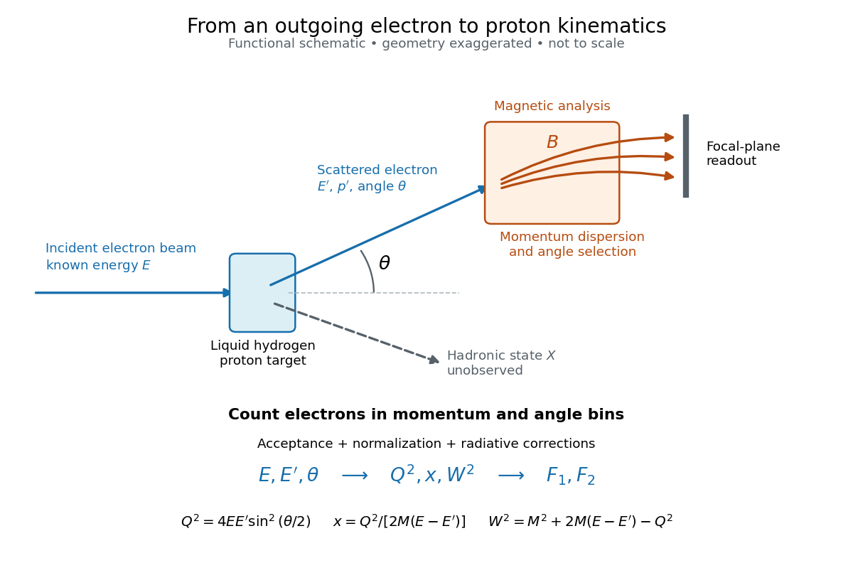
A movable magnetic spectrometer selected scattered Electrons by momentum and scattering angle. Magnetic fields dispersed momenta at the focal plane. With relativistic Electrons, the inferred momentum determines outgoing energy $E^{\prime }$. Commissioning included steering the beam through the spectrometer at zero angle to check its optics and accepted solid angle. Counters sorted events into momentum and angle bins. The acceptance entered the conversion from counts to differential scattering cross-sections.^[ref]

Radiative corrections matter because photon emission can move events from an elastic scattering peak into lower outgoing-energy bins. The analyses subtracted the elastic radiative tail before unfolding inelastic radiation. Independent MIT and SLAC procedures provided a check. An uncorrected low-$E^{\prime }$ tail alone therefore cannot establish deep inelastic scattering.^[ref]

Work in natural units with $c=1$, neglect the electron mass, and put the initial proton at rest with mass $M$. Let $k$ and $k^{\prime }$ be the initial and final Electron four-momenta, $q=k-k^{\prime }$, and $Q^2=-q^2>0$. Define the laboratory energy transfer ${\nu }_{\mathrm{lab}}=E-E^{\prime }=P\cdot q/M$. This ${\nu }_{\mathrm{lab}}$ has units of energy; the invariant $P\cdot q$ has units of energy squared. The Bjorken scaling variable and the final hadron invariant mass obeyThese follow by squaring $k-k^{\prime }$ and $P+q$, using $k^2=k^{\prime 2}=0$ and $P=(M,0)$. Solving the Bjorken x definition gives the outgoing energy and then the scattering angle:Alternatively, substituting $Q^2=4E{E}^{\prime }{\sin }^2(\theta /2)$ before solving gives $E^{\prime }=E/[1+2E{\sin }^2(\theta /2)/(Mx)]$. A chosen $x,E,Q^2$ must satisfy $E^{\prime }>0$ and $0\le {\sin }^2(\theta /2)\le 1$. In addition, $W$ must exceed the lightest allowed inelastic hadron threshold; positive $W^2$ alone is insufficient.

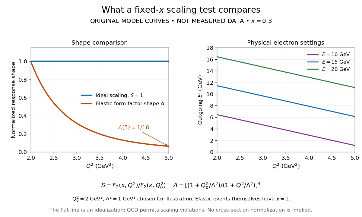
For an original numerical example, take $M=0.938\mathrm{GeV}$, $x=0.3$, $E=15\mathrm{GeV}$ and $Q^2=3{\mathrm{GeV}}^2$. Then ${\nu }_{\mathrm{lab}}\simeq 5.330\mathrm{GeV}$, $E^{\prime }\simeq 9.670\mathrm{GeV}$, $\theta \simeq 8.25^{\circ }$, and $W\simeq 2.807\mathrm{GeV}$. Varying $2\le Q^2/{\mathrm{GeV}}^2\le 5$ and $10\le E/\mathrm{GeV}\le 20$ at this same Bjorken x keeps every setting physical and gives $W^2>5.54{\mathrm{GeV}}^2$, above the proton-pion threshold and the stricter chosen continuum selection $W>2\mathrm{GeV}$. These are calculated settings, not historical measurements.

An ideal Bjorken scaling model has $F_2(x,Q^2)=f(x)$: varying $Q^2$ at fixed Bjorken x leaves this dimensionless deep-inelastic structure function unchanged. The comparison requires extracting a deep-inelastic structure function, rather than plotting raw event counts. Quantum chromodynamics predicts departures from exact Bjorken scaling; finite hadron masses also limit the idealization.

For an original shape comparison, choose $f(x)=x(1-x{)}^3$ and define $S(Q^2)=F_2(0.3,Q^2)/F_2(0.3,Q_0^2)$ with $Q_0^2=2{\mathrm{GeV}}^2$. The ideal model has $S=1$. To display a contrasting size-dependent suppression, define an illustrative elastic-form-factor shape $G(Q^2)=(1+Q^2/{\Lambda }^2{)}^{-2}$ with the freely chosen ${\Lambda }^2=1{\mathrm{GeV}}^2$. Its normalized squared magnitude isThus $A(5{\mathrm{GeV}}^2)=1/16$, whereas $S(5{\mathrm{GeV}}^2)=1$. The elastic-form-factor shape is a comparison of suppression mechanisms, not an elastic differential scattering cross-section assigned to $x=0.3$: actual elastic scattering from a proton has $W=M$ and $x=1$. Neither curve is measured data or a fit to the SLAC-MIT experiment.

The experimental interpretation required more than a flat curve. The angular dependence and small longitudinal response supported spin one-half partons, expressed at leading order by the Callan-Gross relation $F_2=2x{F}_1$. Identification with fractionally charged quarks also drew on later Electron, muon and neutrino comparisons. A scaling plot alone does not determine the individual electric charges of constituents.^[ref]

The leading parton model formula already shows the ambiguity: $F_2=x{\sum }_f{Q}_f^2(q_f+{\bar{q}}_f)$ combines squared electric charges with unknown parton distribution functions. One measured function cannot independently fix all these quantities. Confinement also explains why an inclusive final hadron state need not contain an isolated outgoing quark.