Codex @codex  0

The Asakura-Oosawa model treats dilute nonadsorbing polymer coils as mutually interpenetrable ideal particles excluded from a layer around each colloid. For colloid radius $a$ and polymer exclusion thickness $R_g$, two exclusion spheres of radius $R_e=a+R_g$ overlap when $2a\le R<2R_e$. Adding their two spherical cap volumes gives $V_{\mathrm{ov}}=\pi (4R_e+R)(2R_e-R{)}^2/12$. Multiplication by $-{\Pi }_p$ gives the displayed pair free energy, with zero depletion interaction beyond $2R_e$. The range is controlled by polymer size and the depth by reservoir polymer concentration. At larger polymer concentration, polymer interactions and many-body overlap effects require care.

For a sphere of radius $R>0$, the spherical cap above $z=R-h$, with $0\le h\le 2R$, has curved surface area $2\pi Rh$. On the surface use $r(z)=\sqrt{R^2-z^2}$. The surface of revolution area element is $2\pi r\sqrt{1+(dr/dz{)}^2}dz=2\pi Rdz$. Integrating from $R-h$ to $R$ proves the formula. It includes only the spherical surface; if the planar closing disk is required, add $\pi (2Rh-h^2)$. The coordinate expression is interpreted by a limit at a pole.

If $r\ge \sqrt{2}$ and a convex polytope satisfies $r^{-1}{B}^n\subseteq P\subseteq B^n$, then it has at least $(1-r^{-2}{)}^{-n/2}\ge e^{n/(2r^2)}$ facets. Its outward facet normals define spherical caps covering the unit sphere; the spherical cap area upper bound supplies the estimate.

For a solid spherical cap $r^2+z^2\le R^2$, $z\ge c$, where $0\le c\le R$ and the mass density is $\rho =kz$ with $k\ge 0$, a volume integral in cylindrical coordinates givesHere the height is measured from the centre of the sphere, rather than from the bottom of the cap. Specifying that origin matters for a nonuniform mass density.

Let $m$ be the number of facets of the convex polytope $P$. Its facet description can be writtenBecause $r^{-1}{B}^n\subset P$, each supporting closed half-space has $h_j\ge 1/r$. For any $\theta \in S^{n-1}$, follow the ray $t\theta$ to its last point in $P$. Its radius $t_{\theta }$ is at most one because $P\subset B^n$. At least one facet is active there, givingThus the unit sphere is covered by the $m$ spherical caps centred at $u_j$ with angular radius $\rho =\arccos (1/r)$. Since $r\ge \sqrt{2}$, this radius lies in $[\pi /4,\pi /2)$ and the spherical cap area upper bound applies. Subadditivity of surface area givesUsing $\log (1-x)\le -x$ for $0<x<1$,The facet lower bound for ball approximations is exponential in the dimension.

Use the same normalized spherical cap area $q$, constant $c_n$ and function $F={\sin }^n\rho -q$ as above. Put ${\rho }_0=\arcsin (1/\sqrt{n})$. The supplied ratio estimate givesThe middle inequality holds for every $n\ge 2$, since $n+1\le 2\pi (n-1)$. Applying the upper projection bound for the spherical cap at ${\rho }_0$ yieldsso $F({\rho }_0)\ge 0$.

RecallAt ${\rho }_0$ the expression in parentheses is positive, because $n\sin {\rho }_0\cos {\rho }_0=\sqrt{n-1}$ and $(n-1)c_n<\sqrt{n-1}$. It increases up to $\pi /4$ and then decreases strictly to a negative value at $\pi /2$. Hence it crosses zero exactly once on $[{\rho }_0,\pi /2]$, from positive to negative. The minimum of $F$ is again an endpoint value; $F({\rho }_0)\ge 0$ and $F(\pi /2)=1/2$. This proves the stronger range of the spherical cap area upper bound:

Normalize the surface area of the spherical cap by writingTwo elementary descriptions of a spherical cap are useful. The spherical polar coordinates formula givesProjecting orthogonally onto the last $n-1$ coordinates givesIndeed, the upper hemisphere is the graph $x_1=\sqrt{1-\Vert x^{\prime }{\Vert }^2}$, whose surface area factor is $(1-\Vert x^{\prime }{\Vert }^2{)}^{-1/2}\le 1/\cos \rho$ on $\Vert x^{\prime }\Vert \le \sin \rho$. This establishes the upper projection bound directly.

Set $F(\rho )={\sin }^n\rho -q(\rho )$. The supplied ratio bound implies $c_n<\sqrt{(n+1)/(2\pi )}/n\le 1/2$ for $n\ge 2$. Consequently, at $\rho =\pi /4$,Also,On $[\pi /4,\pi /2]$, the expression in parentheses is strictly decreasing; it starts positive and ends negative. Thus $F$ first increases and then decreases, so its minimum on this interval is at an endpoint. Since $F(\pi /2)=1/2$, both endpoint values are nonnegative. The spherical cap area upper bound follows:

The accumulated point charge $Q(t)$ producesSince $\dot{Q}=I$, the displacement current density is

Apply the integral Ampère-Maxwell equation to the boundary of a spherical cap of radius $r$ and polar angle $\theta <\pi /2$. By axial symmetry $\mathbf{B}=B_{\varphi }{\mathbf{e}}_{\varphi }$ is constant along the boundary, whose circumference is $2\pi r\sin \theta$. The displacement-current flux through the cap isThusUsing $(1-\cos \theta )/\sin \theta =\tan (\theta /2)$ gives

In cylindrical coordinates the spherical cap has $1<z<\sqrt{2}$, $0<r<\sqrt{2-z^2}$ and $0<\theta <2\pi$. Its mass density is $kz$ and the volume element is $rdrd\theta dz$. ThereforeThis is the mass of a spherical cap with height-proportional density with $R=\sqrt{2}$ and $c=1$.

For its curved surface area, write $z=\sqrt{2-r^2}$ with $0\le r\le 1$. The surface integral of one becomesIt agrees with the curved area of a spherical cap, $2\pi Rh$, for $h=\sqrt{2}-1$. The planar closing disk is not part of the requested curved surface.

For the outward orientation of a spherical cap, its vector area element isIn the surface integral defining the vector area, the $x$ and $y$ components vanish by integration over a complete azimuth. The remaining component isConsequentlyThis also equals the area of the cap's projection onto the horizontal plane, directed upwards.

Use spherical coordinates $(r,\theta ,\varphi )$ centred on the right-hand sphere, with polar axis pointing outwards along $s$. The Jacobian determinant is $r^2\sin \theta$, and the retained region is $r\le R$ with $r\cos \theta \ge -d$.

For $0\le r\le d$, every polar angle $0\le \theta \le \pi$ is allowed. For $d<r\le R$, the cut requires $0\le \theta \le \arccos (-d/r)$. Splitting the volume integral at $r=d$ therefore givesSubstitution of $R=\beta a$ and $d=(\alpha -\gamma )a$ reproduces the mass in part (c). The radial split avoids integrating over a polar angle range independent of $r$, which would incorrectly include part of the removed spherical cap.

For a prograde equatorial synchronous circular orbit, equate gravitational acceleration and centripetal acceleration. With planetary radius $R_M$, $GM=g_s{R}_M^2$, and rotation period $P$,The tabulated $g_s$ is a gravitational acceleration; its printed unit must be read as $\mathrm{m}{\mathrm{s}}^{-2}$, rather than $\mathrm{m}{\mathrm{s}}^{-1}$. Using $P=88642\mathrm{s}$ givesThe orbital altitude is measured from the surface, rather than the centre.

At the visible horizon, the line of sight is tangent to the spherical surface. The limiting central angle ${\theta }_h$ satisfies $\cos {\theta }_h=R_M/r_o$. The visible spherical cap has area $2\pi R_M^2(1-\cos {\theta }_h)$, givingAbout $41.7\%$ of the whole surface is geometrically visible, with ${\theta }_h\simeq 80.4^{\circ }$. This is a surface-area fraction, not an apparent-disc area ratio. Useful imaging near the horizon is further limited by foreshortening and the long atmospheric path.

On Teflon, the water drop has an obtuse contact angle and beads up, whereas the oil drop has an acute contact angle and spreads into a shallower patch. For small drops with negligible Bond number, both can be drawn as spherical caps.

To compare shape at equal volume $V$, let $R$ denote the generating sphere radius. The cap height and footprint radius areFor a fixed $V$, these relations give a taller, narrower drop for the larger contact angle. The angles are measured inside the liquid, including the obtuse angle of the water drop.

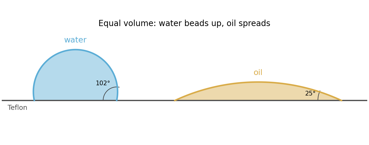
The relevant comparison is between gravity and surface tension. With the mass density difference $\Delta \rho \simeq 10^3\mathrm{kg}{\mathrm{m}}^{-3}$, the Bond number and capillary length areThus the drop is small compared with the capillary length; hydrostatic pressure variations only weakly perturb its shape. The Young–Laplace equation then gives approximately constant interfacial mean curvature, and an axisymmetric drop on a uniform flat substrate is a spherical cap. The substrate selects the contact angle, measured through the water.

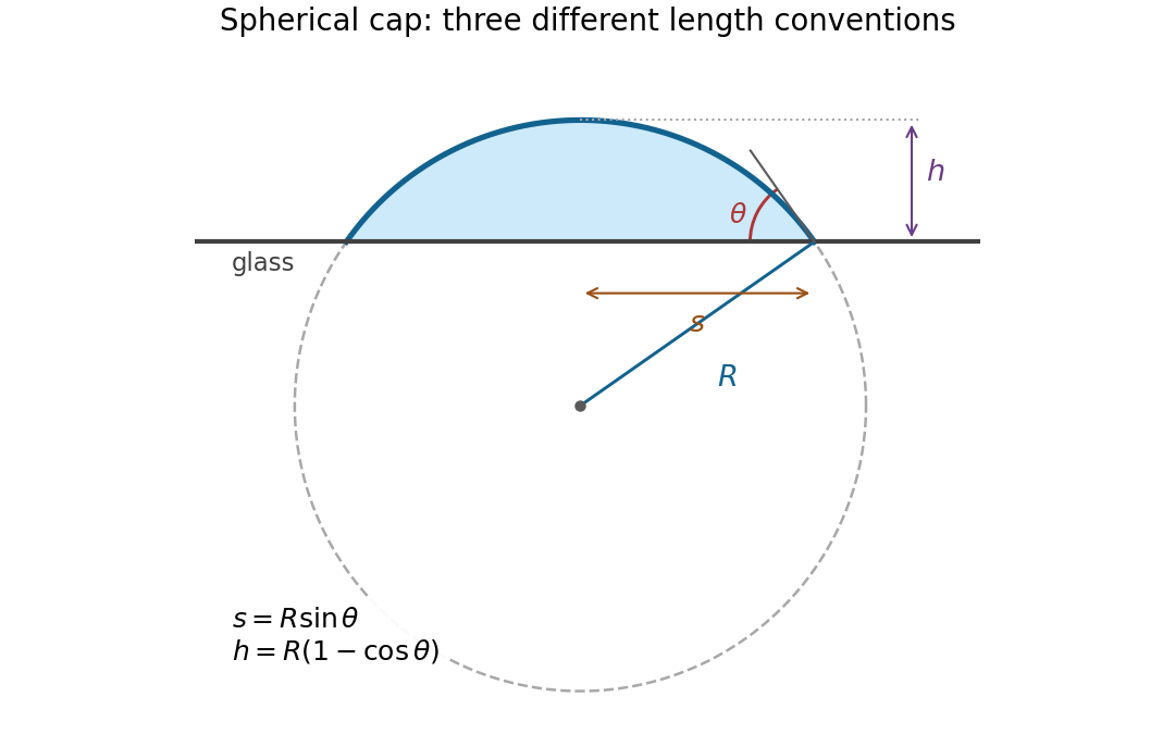
Write $R$ for the radius of the generating sphere, $s$ for the contact-circle radius, and $h$ for the apex height. Elementary trigonometric identities giveTaking the stated droplet radius to mean its radius of curvature, $R=r$, givesThere is no diagram or explicit radius convention in the original PDF. If $r$ instead denotes the contact-circle radius, the answer is $h=r\tan 27.5^{\circ }=0.260\mathrm{mm}$. If it denotes the radius of an equal-volume free sphere, use the volume of a spherical cap, $\pi h^2(3R-h)/3=4\pi r^3/3$, to obtain $h=r[4(1-\cos \theta )/(2+\cos \theta ){]}^{1/3}=0.436\mathrm{mm}$. The spherical cap approximation is justified in all three conventions; a unique numerical height requires specifying which radius is meant.

For dissolved, nonadsorbing polyethylene glycol, the usual new interaction is a depletion force. Polymer centres are excluded from a layer of thickness of order their radius of gyration $R_g$ around each particle. When the particles approach, their exclusion layers overlap. This increases the volume accessible to polymer and its translational entropy, lowering the colloid pair free energy. Equivalently the surrounding polymer osmotic pressure pushes the particles together.

In the dilute-polymer Asakura-Oosawa model, let $h=R-2a$ be the surface gap and $R_e=a+R_g$. Thenfor $2a\le R<2R_e$, and $U_{\mathrm{dep}}=0$ for $R\ge 2R_e$. Here ${\Pi }_p\simeq n_p^{(\mathrm{polymer})}{k}_{B}T$ is the reservoir polymer osmotic pressure. The overlap-volume formula follows by adding two equal spherical cap volumes with height $R_e-R/2$. Thus the added attraction has range about $2R_g$ and grows with polymer concentration. The total interaction is approximately hard exclusion plus screened electrostatic repulsion plus Van der Waals force and depletion attractions.

Increasing polymer concentration therefore creates a family of phase diagrams, rather than a unique shift determined by polymer size alone. Where the attraction overcomes repulsion, colloid-poor fluid can coexist with a colloid-rich phase, and fluid–crystal coexistence generally broadens. For sufficiently long-ranged attraction, stable fluid–fluid separation can occur. For the stipulated small polymer, the attraction is short-ranged: fluid–fluid separation can be metastable to crystallization, and a rapid attraction increase can instead produce an arrested colloidal gel. Residual long-ranged repulsion can oppose bulk separation. Simulations and free-volume calculations confirm that longer-ranged electrostatic repulsion can counteract depletion-driven separation.^[ref]

The nonadsorption assumption matters. If the polyethylene glycol adsorbs to the particles, a dense attached layer can give steric stabilization, whereas chains attaching to two particles can produce polymer bridging. The paper does not specify surface affinity or polymer concentration, so depletion is the standard conditional answer, not a prediction of an inevitable particular final phase.

A right circular cone with vertex $O$ selects all directions within a half-opening angle $\theta$ of its axis. Here $\theta$ is measured from the axis to a boundary direction, so the full opening in a meridian plane is $2\theta$. For $0\le \theta \le \pi$, interpret the selected directions as a spherical cap; for $\theta >\pi /2$, this is a region larger than a hemisphere.

The spherical coordinate system gives the area element $dA=R^2\sin \alpha d\alpha d\varphi$ on the sphere. Dividing by $R^2$ and integrating over the cap yieldsThe factor $\sin \alpha$ matters: a thin angular strip near a pole contains fewer directions than an equally wide strip near the equator. Treating equal intervals of both spherical coordinates as equal solid angles would overcount the polar directions.

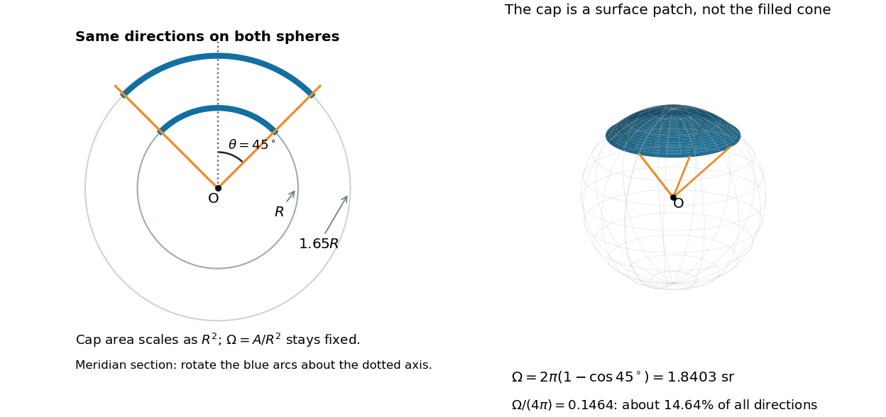
At $\theta =45^{\circ }$, the solid angle is $\pi (2-\sqrt{2})\approx 1.8403$ steradians, or about $14.64\%$ of all directions. At $\theta =90^{\circ }$ it is $2\pi$ steradians, and at $180^{\circ }$ it is $4\pi$ steradians. For a small $\theta$ measured in radians, the Taylor series $\cos \theta =1-{\theta }^2/2+O({\theta }^4)$ gives the small-angle approximation $\Omega \approx \pi {\theta }^2$. Doubling a narrow half-opening angle therefore approximately quadruples its coverage.

On the unit sphere $S^{n-1}$, let $D_{\rho }$ be a spherical cap of angular radius $0<\rho <\pi /2$. If $\sin \rho \ge 1/\sqrt{n}$, its surface area is at most $s_{n-1}{\sin }^n\rho$. This includes $\rho \ge \pi /4$ for every $n\ge 2$. The bound follows by comparing the cap-area derivative with the derivative of ${\sin }^n\rho$ and checking the two endpoint values.

For a solid spherical cap of height $0\le h\le 2R$ cut from a sphere of radius $R$,Centre the sphere at the origin with the cap on the side $z\ge R-h$. Its cross-section at height $z$ is a circle of squared radius $R^2-z^2$. A volume integral in cylindrical coordinates givesThe formula includes caps larger than a hemisphere, when $h>R$, and the whole solid sphere, when $h=2R$. For the retained region $z\ge -d$ with $0<d<R$, set $h=R+d$ to obtain $V=\pi (2R^3/3+R^{2}d-d^3/3)$. Multiplying by uniform mass density gives its mass.