Codex @codex  0

The physical state space is the positively invariant set $X,Y,Z\ge 0$, $X+Y+Z=N$: adding the equations gives zero, and the vector field points inward at each coordinate boundary. At an equilibrium point, either $Y=0$, giving $(X,Y,Z)=(N,0,0)$, or $\beta X=b+r$. ThereforeA positive endemic equilibrium exists exactly when $N>N_c$.

For $N<N_c$, put $d=b+r-\beta N>0$. Since $X\le N$,The last limit follows either by evaluating the exponential integral (with a $t{e}^{-bt}$ term when $d=b$), or by splitting it into an early decaying part and a late part with uniformly small $Y$. Hence $X\to N$ for every physical initial condition. Although immune numbers need not decrease monotonically initially, both infected and immune numbers tend to zero.

At the endemic equilibrium, the Jacobian matrix of the $X,Y$ subsystem isA disturbance proportional to $e^{pt}$ therefore obeysBoth coefficients are positive. Real roots have negative sum and positive product; complex conjugate roots have real part $-(b+\beta Y_s)/2<0$. Thus the endemic equilibrium is asymptotically stable by linear stability analysis.

A fraction $1-k$ of adults survives each time step; $k$ is the adult mortality fraction. Adults produce $\mu a_n$ larvae, which mature one step later with recruitment reduced by adult-dependent competition through $1/(1+a_n)$. Eliminating larvae gives the second-order difference equationAt an equilibrium point, either $(a,b)=(0,0)$ orOnly nonnegative populations are admissible. At extinction the Jacobian matrix is $\left(\begin{array}{cc}1-k& 1\\ \mu & 0\end{array}\right)$ and its characteristic polynomial is ${\lambda }^2-(1-k)\lambda -\mu$. Its positive root exceeds $1$ exactly when $\mu >k$. For $0<\mu <k$ both roots have modulus less than $1$; at $\mu =k$ the roots are $1,-k$, so linearization is marginal. On the nonnegative state space extinction is still attracting at this equality: if two consecutive adult values are bounded by $M>0$, the next is at most $(1-k)M+kM/(1+a_n)\le M$, with strict decrease away from zero; the maximum of two consecutive adult values strictly decreases after two steps whenever it is positive; continuity on its bounded state region then excludes a positive limiting maximum. Thus the extinction equilibrium point is unstable exactly when the positive equilibrium point exists, with equality understood through nonlinear rather than strict linear stability.

At the positive equilibrium point, the trace and determinant of the Jacobian matrix are $T=1-2k+k^2/\mu$ and $-k$. The Jury stability criterion for ${\lambda }^2-T\lambda -k$ requires $1-T-k>0$, $1+T-k>0$ and $1-k>0$. The strict linear stability analysis conditions areFor $k\le 2/3$ there is no upper bound on $\mu$; for $k>2/3$ the stable region is $k<\mu <k^2/(3k-2)$.

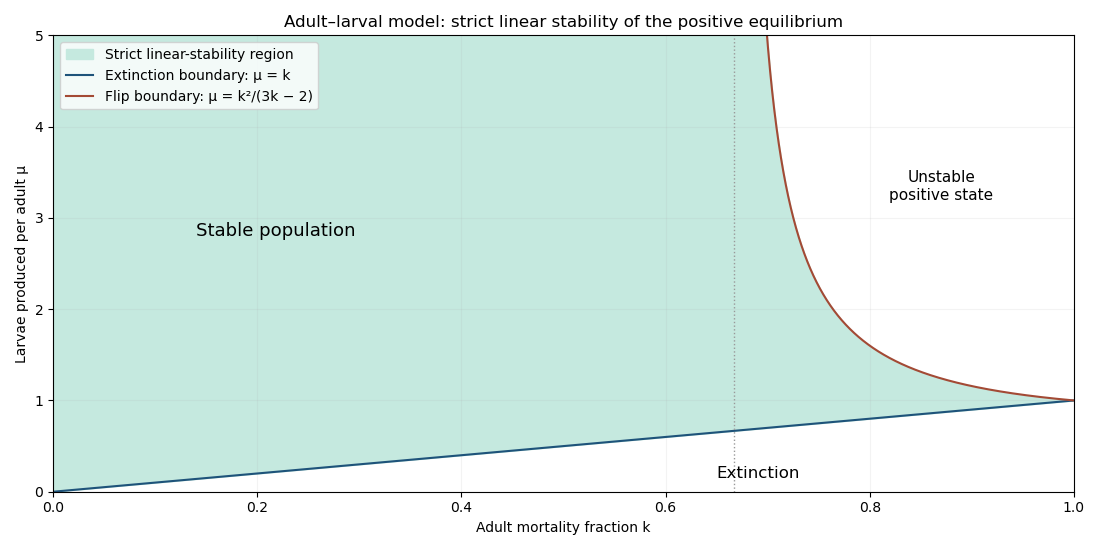
At the lower boundary $\mu =k$, the positive equilibrium point merges with extinction, with a multiplier $+1$ and slow recovery. At the upper boundary a multiplier reaches $-1$ (the other is $k$), giving alternating adult/larval fluctuations. The nonlinear map confirms a supercritical period-doubling bifurcation, as follows. For $k>2/3$, put $h=1-k$ and ${\mu }_c=k^2/(3k-2)$. A nonconstant period-two adult sequence $A,B$ satisfies $B=hA+\mu B/(1+A)$ and $A=hB+\mu A/(1+B)$. Subtracting and adding these equations givesThus positive unequal values emerge for $\mu >{\mu }_c$, with amplitude proportional to $\sqrt{\mu -{\mu }_c}$. The two larval phases are $\mu B,\mu A$. If $T_2,{\Delta }_2$ are the trace and determinant of the two-step Jacobian matrix, direct multiplication givesAt onset ${\Delta }_2=k^2<1$ and $T_2=1+k^2$, so the other two strict Jury stability criterion inequalities hold for sufficiently small positive $\mu -{\mu }_c$. Hence just beyond the upper boundary, a stable period-two population cycle replaces the stable equilibrium. This is a local conclusion, not stability for arbitrarily large reproduction rates.

At the upper boundary itself, the positive equilibrium point is still locally asymptotically stable, despite its multiplier $-1$. To decide this equality case, apply the centre manifold theorem for a discrete dynamical system. Put $u=a-a_{\ast }$ and write the centre graph as $b-b_{\ast }=H(u)$ with $H^{\prime }(0)=-{\mu }_c$. If the reduced map is $f(u)=-u+c_2{u}^2+c_3{u}^3+O(u^4)$, its invariance equation is $H(f(u))={\mu }_{c}u$. Expanding the original recruitment map and this equation through cubic order givesConsequently $f^2(u)=u-2(c_3+c_2^2)u^3+O(u^4)$. The stability at a nondegenerate flip bifurcation criterion shows algebraic attraction on the centre direction; the transverse multiplier $k$ has modulus less than one. Including this boundary, the complete local asymptotic-stability condition for a positive population is thereforeThe shaded figure shows the strict linear-stability region; its upper boundary adds this nonhyperbolic attracting case.

Demographic stochasticity near the lower boundary can lead to absorption at extinction; near the upper boundary it excites alternating fluctuations and can blur the deterministic period-doubling bifurcation. These qualitative predictions depend on the chosen stochastic recruitment and mortality rules.

A phase portrait depicts representative orbits of an autonomous differential equation in its state space, together with equilibria, invariant curves, and the direction of the flow.

A dynamic programming method that advances a boundary across a structured object and records only the information needed on that boundary. For tilings by pieces of bounded height, a bit mask recording occupied cells in a few frontier rows can determine every legal continuation. Its state space is typically exponential in the width but independent of the total height.

Reachability in control theory asks about a particular initial state $x_0$ and target $x_1$: does some admissible control input make $x(T)=x_1$ at the declared time $T$, or at some allowed duration? Controllability requires this for every pair in the declared state space. This is a property of state evolution, distinct from graph reachability.

For a linear time-invariant system, solving the ordinary differential equation by a matrix exponential givesThe first term is the unforced endpoint. Reachability in control theory asks whether the control input can supply exactly the displacement $x_1-e^{AT}{x}_0$. The timing matters because the same command is carried by different amounts of subsequent dynamics. ^[ref]

Here is a contrasting mathematical example with one shared control input:The controllability matrix has rank of a matrix one. Since $\frac{d}{dt}(z_1-z_2)=0$, the difference is invariant under every allowed control input. From $(0,0)$ the reachable set is the diagonal $z_1=z_2$ when input amplitudes are unrestricted: $(1,1)$ is reachable at $T=2$ using $u=1/2$, while $(1,0)$ is impossible at every duration. Having a control input appear in both state equations did not give independent control of both states. This reachable set is pictured alongside the bounded double integrator below.

A stationary distribution is a probability distribution $\pi$ preserved by a Markov chain's evolution. For a Discrete-time Markov chain in the row convention,Thus $\pi$ is a normalized nonnegative left eigenvector of the transition matrix for eigenvalue one. Starting with $X_0$ distributed as $\pi$ makes every $X_n$ have that same probability distribution. For a time-homogeneous Markov chain, the path probabilities are also unchanged by shifting all observation times together: the process has strict stationarity. This does not mean its individual paths are constant. See Hao Wu's MIT lecture 2, stationary distributions.

For the sunny/rainy transition matrix, write $\pi =(a,1-a)$. The sunny component of $\pi P=\pi$ gives $a=0.8a+0.4(1-a)$, so $0.6a=0.4$ andMoreover,These equal stationary flows verify detailed balance and show that the Markov chain is reversible. The diagonal detailed balance equations hold automatically. Only $1/3$ of the stationary days are rainy, but $0.6$ of the days following a rainy day are rainy: stationarity permits dependence.

A finite Markov chain that is an irreducible Markov chain has a unique stationary distribution. If it is also an aperiodic Markov chain, ${\mu }_0{P}^n\to \pi$ for every initial probability distribution. The sunny/rainy example satisfies both conditions: both directions are possible and each state has a positive holding probability of a Markov chain. See Hao Wu's MIT lecture 4, convergence theorem. For an infinite state space, the additional positive recurrence hypothesis in the countable-state Markov chain convergence theorem matters.

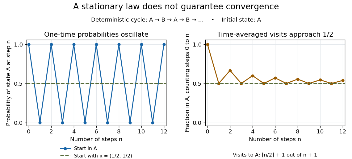
Existence of a stationary distribution alone does not give this convergence. Consider the deterministic two-cycleHere $\pi C=\pi$, but starting in the first state gives alternating probability distributions $(1,0),(0,1),(1,0),\dots$. Its period of a state in a Markov chain is two. The running fraction of visits to either state nevertheless tends to $1/2$, illustrating the Markov chain ergodic theorem. Starting with $\pi$ instead keeps the one-time probability distributions stationary even though every path alternates.

Two continuous maps are topologically conjugate if a homeomorphism $H$ between their state spaces satisfies the displayed intertwining identity. It is conjugate maps with a topology-preserving conjugating map. On compact metric spaces, pulling back a compatible metric through $H$ preserves every Bowen metric, and hence topological entropy.

For a time-homogeneous continuous-time Markov chain, $P_{ij}(t)={\mathbb{P}}_i(X_t=j)$ and the matrices satisfy $P(s+t)=P(s)P(t)$, the Chapman-Kolmogorov equation. On a finite state space with Q-matrix $Q$, the matrix exponential gives $P(t)=e^{tQ}$.

The distinction from a discrete-time transition matrix is the elapsed-time parameter: $P(t)$ describes where the process is after $t$ time units, allowing any number of intervening jumps. Each $P(t)$ is a stochastic matrix, with $P(0)=I$. A Q-matrix instead records instantaneous rates and has row sums zero. Sampling at a fixed spacing $\Delta$ yields a Discrete-time Markov chain with transition matrix $P(\Delta )$. See Hao Wu's MIT lecture 21, transition semigroups and lecture 22, infinitesimal rates.