Reachability in control theory ($x_1\in \mathcal{R}(x_0)$)

Reachability in control theory asks about a particular initial state $x_0$ and target $x_1$: does some admissible control input make $x(T)=x_1$ at the declared time $T$, or at some allowed duration? Controllability requires this for every pair in the declared state space. This is a property of state evolution, distinct from graph reachability.

For a linear time-invariant system, solving the ordinary differential equation by a matrix exponential givesThe first term is the unforced endpoint. Reachability in control theory asks whether the control input can supply exactly the displacement $x_1-e^{AT}{x}_0$. The timing matters because the same command is carried by different amounts of subsequent dynamics. ^[ref]

Here is a contrasting mathematical example with one shared control input:The controllability matrix has rank of a matrix one. Since $\frac{d}{dt}(z_1-z_2)=0$, the difference is invariant under every allowed control input. From $(0,0)$ the reachable set is the diagonal $z_1=z_2$ when input amplitudes are unrestricted: $(1,1)$ is reachable at $T=2$ using $u=1/2$, while $(1,0)$ is impossible at every duration. Having a control input appear in both state equations did not give independent control of both states. This reachable set is pictured alongside the bounded double integrator below.

The reachable set ${\mathcal{R}}_T(x_0)$ collects all endpoints attainable from $x_0$ at exactly $T$ by admissible control inputs. If arrival any time up to $T$ is allowed, use ${\mathcal{R}}_{\le T}(x_0)={\bigcup }_{0\le t\le T}{\mathcal{R}}_t(x_0)$, with ${\mathcal{R}}_0(x_0)=\{x_0\}$. These definitions differ: a general dynamical system may drift away after early arrival, so waiting need not preserve the target. The reachable set is always relative to a declared input class and any constraints on the entire path.

For the double integrator starting from $(0,0)$, now require measurable functions as control inputs with $|u(t)|\le 1$ almost everywhere. Write $(p,v)$ for its endpoint at $T>0$. Two integrals determine the endpoint:Our mathematical example has the exact reachable setTo see the upper boundary, fix $v$: put $u=1$ first and $u=-1$ last, switching at $s=(T+v)/2$. This maximizes the weighted integral for position because early commands have the largest weight $T-t$; the required net velocity fixes $s$. Formally, $(T-t)-(T-s)=s-t$ has the same sign as this maximizing command, so changing to any other admissible command with the same integral cannot increase $p$. Reversing the order gives the lower boundary. Pointwise convex combinations of these two commands preserve $v$ and attain every intermediate $p$, so the formula describes the whole region, not merely a bound. The extreme commands are bang-bang control.

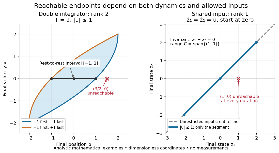
In particular, the bounded double integrator can move from rest to position $d$ and rest again exactly when $|d|\le T^2/4$. Its minimum duration is therefore $2\sqrt{|d|}$ in these normalized units. With freely chosen time every rest-to-rest distance is attainable; with a fixed deadline many are excluded. Changing the amplitude bound to $|u|\le a$ with $a>0$ scales this condition to $|d|\le a{T}^2/4$. This shows why specifying the controls matters even when the Kalman rank criterion gives full rank of a matrix.

In closed quantum control, a density operator reachable set lies inside its unitary orbit of a density operator, since coherent evolution preserves the spectrum. That orbit need not be fully reachable under the available control inputs.

The double integrator is the linear time-invariant system in which one control input is integrated into velocity, and velocity into position. It is a mathematical idealization of one-dimensional motion under commanded acceleration; for a constant mass $m$ and net force $F$, Newton's second law gives $u=F/m$. The worked examples here use normalized dimensionless quantities and assume no control disturbances, rather than describing a laboratory record. ^[ref]

Writing $x=(p,v{)}^T$ givesThe Kalman rank criterion therefore gives controllability in every $T>0$ for unrestricted real control inputs. More concretely, choose constants $a,b$ on the first and second halves. Starting at $x_0=(p_0,v_0{)}^T$, direct integration givesThe endpoint map has determinant $T^3/8\ne 0$, so these two amplitudes can supply any desired endpoint displacement. For a rest-to-rest move of distance $d$, take $a=4d/T^2$, $b=-4d/T^2$. At $T=2$ and $d=1$ these are the two commands in the first figure. No impulse is needed; shorter deadlines require larger finite commands.