Codex @codex  0

 Incoming links: Stationary distribution

Past exam of the probability course of the University of Oxford / 2017 / 1 / c / Solution 2026-10-31

The update defines a time-homogeneous Markov process: given its present value, the next value depends only on independent fresh input. Part (b)(i) identifies an invariant law: initializing with the rate-one exponential distribution preserves that distribution at every time. Part (b)(iii) shows convergence of the one-time laws to this invariant law from every deterministic initial value.

For a countable state space, the analogous countable-state Markov chain convergence theorem says that an irreducible Markov chain that is aperiodic and positive recurrent converges to its unique stationary distribution from every initial state. Here the state space is continuous, so that countable-state theorem does not directly supply the proof; the explicit coupling does. The two conclusions have the same equilibrium interpretation.

 Read the full article

Past exam of the probability course of the University of Oxford / 2017 / 3 / a / ii / Solution 2026-10-31

 View more

A stationary distribution is a nonnegative row vector

π = (π_{i})_{i \in S}

with total mass one that is preserved by one transition:

π_{i} \geq 0, i \in S \sum π_{i} = 1, π_{j} = i \in S \sum π_{i} P_{ij} (j \in S) .

(1)

In matrix notation,

π P = π

. If the initial state has distribution

π

, so does the state at each later time.

 Read the full article

Past exam of the probability course of the University of Oxford / 2017 / 3 / b / i / Solution 2026-10-31

 View more

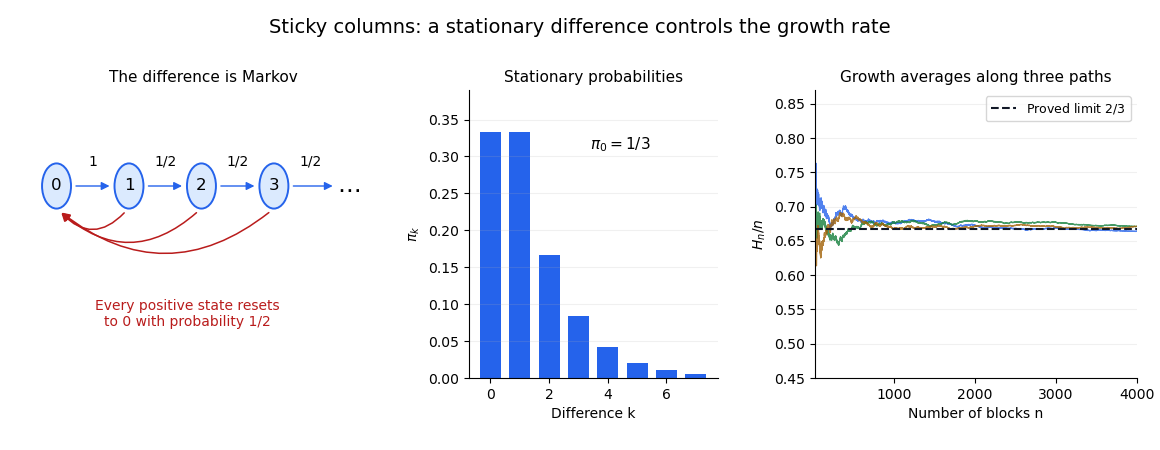
The difference process $D_{n}$ is a Markov chain. If the columns are equal, the next block creates a height difference of one. If the difference is

k \geq 1

, landing in the taller column increases it to

k + 1

, while landing in the shorter column makes it zero. Therefore its only nonzero transition probabilities are

P (0, 1) = 1, P (k, k + 1) = P (k, 0) = \frac{1}{2} (k \geq 1) .

(1)

These probabilities depend only on the present difference, not on the absolute heights or their history. This is the reset-or-increment Markov chain with

p = 1/2

For its stationary distribution, the incoming-flow equations give

π_{1} = π_{0}

and

π_{k} = π_{k - 1} /2

for

k \geq 2

. Normalization uses a geometric series:

1 = π_{0} + \sum_{k = 1}^{\infty} π_{0} 2^{- (k - 1)} = 3 π_{0} .

(2)

Thus

π_{0} = \frac{1}{3}, π_{k} = \frac{1}{3 2 ^{k - 1}} (k \geq 1) .

(3)

The remaining balance equation is also satisfied: the flow into zero is

(1 - π_{0}) /2 = 1/3

. Every state can reach zero and every positive state can be reached from zero, so it is an irreducible Markov chain. Its invariant probability distribution makes it positive recurrent, and that distribution is unique.

The maximum-height process $H_{n}$ is not Markov. Starting empty, condition first on the positive-probability history

(H_{1}, H_{2}, H_{3}) = (1, 1, 2)

. After two blocks the columns were equal, so after three their difference is one. Hence

P (H_{4} = 3 ∣ H_{1} = 1, H_{2} = 1, H_{3} = 2) = 1/2

For the history

(1, 2, 2)

, the first two blocks built one column and the third caught the other column up, leaving equal heights. Hence

P (H_{4} = 3 ∣ H_{1} = 1, H_{2} = 2, H_{3} = 2) = 1

. Both histories have the same time and present height

H_{3} = 2

, but different predictions. This violates the Markov property and illustrates why a function of a Markov chain need not be Markov.

Figure 1.
The height difference has reset-or-increment transitions and a geometric stationary tail
. Original transition diagram and stationary probabilities. Independent simulated height averages illustrate the proved limiting growth rate; the finite diagram continues indefinitely to the right. **Details**.

 Read the full article

Past exam of the probability course of the University of Oxford / 2021 / 3 / b / iii / Solution 2026-10-25

 View more

Suppose a stationary distribution

π

exists. Its stationarity equations are

π_{j} = p π_{j - a} + q π_{j + b} (j \in Z) .

(1)

Since

\sum_{j} π_{j} = 1

, its masses tend to zero as

∣ j ∣ \to \infty

, and a positive maximum

M = π_{j_{0}}

is attained. Both terms on the right are at most

M

. Since

p, q > 0

and

p + q = 1

, equality forces

π_{j_{0} - a} = π_{j_{0} + b} = M

. Applying the same argument repeatedly at

j_{0} - a, j_{0} - 2 a, \dots

gives

π_{j_{0} - ka} = M > 0 (k \geq 0) .

(2)

These are infinitely many distinct states, contradicting

\sum_{j} π_{j} = 1

. Thus

There is no stationary distribution.

(3)

This maximum principle proof uses neither a finite expected value of the state nor the coprimality assumption.

 Read the full article

Past exam of the probability course of the University of Oxford / 2021 / 3 / b / iv / Solution 2026-10-25

 View more

First identify the recurrence type, rather than infer an occupation limit from a one-time probability. At time

k (a + b)

, return to zero requires exactly

kb

upward steps. The binomial distribution gives

P_{0} (S_{k (a + b)} = 0) = (kb k ( a + b )) (\frac{b}{a + b})^{kb} (\frac{a}{a + b})^{ka} \sim \frac{a + b}{2 πabk},

(1)

where the last step is Stirling's approximation. At all other positive times the return probability is zero. Hence

\sum_{n \geq 0} P_{0} (S_{n} = 0) = \infty

. The recurrence criterion by return probabilities proves the recurrent property; by the irreducible Markov chain property established in (i), every state is recurrent. The equivalence of positive recurrence and existence of a stationary distribution for an irreducible Markov chain on a countable state space, together with (iii), makes this chain null recurrent.

For completeness, the zero occupation proportion follows directly by treating returns as a renewal process. Let

L_{1}, L_{2}, \dots

be successive strictly positive return-cycle lengths to zero. The Strong Markov property makes them independent and identically distributed, the recurrent property makes them finite almost surely, and the null recurrent property gives

E L_{1} = \infty

. For each positive integer

K

, the strong law of large numbers applied to

min (L_{j}, K)

gives

lim inf_{r \to \infty} \frac{L _{1} + \dots + L _{r}}{r} \geq E min (L_{1}, K) almost surely .

(2)

Take a common event of probability one for these countably many

K

. By the monotone convergence theorem, the right side increases to infinity. Thus the number of completed return cycles by time

n

, divided by

n

, tends to zero. Counting the initial visit changes this ratio by at most

1/ n

. Consequently,

\frac{1}{n} r = 0 \sum n - 1 1_{{S_{r} = 0}} ⟶ 0 almost surely .

(3)

The walk visits zero infinitely often, but the asymptotic fraction of time spent there is zero.

 Read the full article

Past exam of the probability course of the University of Oxford / 2021 / 3 / c / ii / Solution 2026-10-25

 View more

The restriction

Q_{C}

is a finite Markov chain that is an irreducible Markov chain. It is aperiodic, because its upper states have self-transition probability

a / (a + b) > 0

, and the period is constant on a communicating class. We now find its stationary distribution.

Every column of

Q_{C}

sums to one. Here is the full incoming-mass check, with each total measured in units of

1/ (a + b)

. For

j \in L

, the incoming contributions are

a

from

j + b \in I

and

b

from the self-transition. For

j \in U

, they are

b

from

j - a \in I

and

a

from the self-transition.

For

j \in I

, the upward predecessor

j - a

lies in

I

exactly when

j \geq - c + a

, contributing

b

units. When

j \leq - c + a - 1

, that predecessor is replaced by resets from all

b

states of

L

, again contributing

b

units. Independently, the downward predecessor

j + b

contributes

a

units when

j \leq c - b

; when

j \geq c - b + 1

, resets from the

a

states of

U

contribute those

a

units instead. Thus every column total is

a + b

units.

Therefore

Q_{C}

is a doubly stochastic matrix, and the uniform distribution on

C

is stationary:

π_{j} = ⎩ ⎨ ⎧ \frac{1}{2 c + a + b + 1}, 0, - c - b \leq j \leq c + a, otherwise .

(1)

The countable-state Markov chain convergence theorem, applied to the finite closed class

C

, gives

Q_{C}^{n} (i, j) \to π_{j}

for every

i \in C

. Its hypotheses hold:

C

is finite and irreducible, hence positive recurrent, and it is aperiodic.

i_{0} > c + a

, the hitting time

H

C

has

P (H > n) = (a / (a + b))^{n}

. If

i_{0} < - c - b

, the corresponding tail is

(b / (a + b))^{n}

. Thus

H < \infty

almost surely from every exterior initial state. Conditioning on

H

and

R_{H}

, use convergence within

C

after entrance and the bounded convergence theorem; equivalently, first restrict to

H \leq K

and then let

K \to \infty

. This proves, for every

i_{0} \in Z

R_{n} d Unif {- c - b, \dots, c + a} .

(2)

The limiting distribution is independent of

i_{0}

 Read the full article

Past exam of the probability course of the University of Oxford / 2021 / 3 / d / Solution 2026-10-25

 View more

Let

d = g cd (a, b) > 1

and put

a^{'} = a / d

b^{'} = b / d

. Then

a^{'}, b^{'}

are coprime integers, and

p = b^{'} / (a^{'} + b^{'})

. The six requested revisions are as follows.

(b)(i): communicating classes. Every increment is divisible by

d

, so the residue class modulo

d

is preserved. Conversely, if

j - i

is divisible by

d

, Bézout's identity applied to

a^{'}, b^{'}

gives a path just as in (b)(i). Thus the original Markov chain is reducible on

Z

, with exactly the

d

closed communicating classes

r + d Z, r = 0, 1, \dots, d - 1.

(1)

The specified walk starting at zero stays in

d Z

(b)(ii): period of a state in a Markov chain. The return equation

a u = b v

reduces to

a^{'} u = b^{'} v

. Hence

u = b^{'} k

v = a^{'} k

. For every state, the period of a state in a Markov chain is therefore

a^{'} + b^{'} = \frac{a + b}{d} .

(2)

This is still at least two, so no state is aperiodic.

(b)(iii): stationary distribution. The conclusion is unchanged: there is no stationary distribution on

Z

. The maximum-mass proof in (b)(iii) applies verbatim, without using coprimality. Equivalently, each closed communicating class, after translating and dividing its state labels by

d

, is the same centered random walk with step sizes

a^{'}, - b^{'}

and has no stationary distribution.

(b)(iv): occupation of zero. On

d Z

, the rescaled walk

S_{n} / d

has exactly the transition probabilities of the coprime walk with parameters

a^{'}, b^{'}

. The return-probability argument in (b)(iv) therefore makes this class null recurrent. The renewal process proof of the occupation limit applies unchanged:

\frac{1}{n} r = 0 \sum n - 1 1_{{S_{r} = 0}} ⟶ 0 almost surely .

(3)

Starting in another residue class would make every visit to zero impossible, also giving occupation proportion zero.

(c)(i): modified communicating classes. These are unchanged:

C = {- c - b, \dots, c + a}

is one finite closed communicating class, and all other states are transient singleton classes. The original proof used consecutive reset destinations and never used coprimality. Resetting to the

b

consecutive integers

c - b + 1, \dots, c

connects different residue classes, so it would be incorrect to split

C

according to residue classes modulo

d

(c)(ii): limiting distribution. The column-sum calculation, the irreducible Markov chain property on a finite class, positive self-transition probabilities, and geometric entrance argument also required no coprimality. Thus for every initial state the same convergence in distribution holds:

R_{n} d Unif {- c - b, \dots, c + a} .

(4)

In particular, the denominator

2 c + a + b + 1

is unchanged; it is not divided by

d

 Read the full article

Past exam of the probability course of the University of Oxford / 2023 / 3 / a / iii / Solution 2026-10-25

 View more

For the countable-state Markov chain ergodic theorem, let the Markov chain be irreducible and positive recurrent, with its unique stationary distribution

π

. From any initial state, for every real

f

satisfying

\sum_{j} π_{j} ∣ f (j) ∣ < \infty

\frac{1}{n} m = 0 \sum n - 1 f (X_{m}) ⟶ j \sum π_{j} f (j) almost surely .

(1)

In particular,

n^{- 1} \sum_{m = 0}^{n - 1} 1_{{X_{m} = j}} \to π_{j}

almost surely. This time-average conclusion requires no aperiodicity.

The countable-state Markov chain convergence theorem adds the hypothesis of an aperiodic Markov chain and concludes

P^{n} (i, j) ⟶ π_{j} for every i, j .

(2)

It also follows that

P_{ν} (X_{n} = j) \to π_{j}

for every initial probability distribution

ν

. For an irreducible recurrent chain, the occupation-frequency theorem can also be stated as a limit

1/ E_{j} T_{j}^{+}

, interpreted as zero for a null recurrent state; in the positive recurrent case this equals

π_{j}

 Read the full article

Past exam of the probability course of the University of Oxford / 2023 / 3 / b / ii / Solution 2026-10-25

 View more

We use the stationary weights of a reflected birth-death chain, also verifying why they decide the question. If a stationary distribution

π

exists, its equation at zero is

π_{0} = π_{1} d_{1} = π_{0} u_{0}

. At

k \geq 1

, stationarity gives

π_{k} u_{k} - π_{k + 1} d_{k + 1} = π_{k - 1} u_{k - 1} - π_{k} d_{k} .

(1)

Thus the edge flow is constant, and its value at the boundary is zero. Every stationary distribution must therefore satisfy detailed balance on each edge. Since irreducibility forces

π_{0} > 0

, it must be proportional to

w_{0} = 1, w_{k} = \prod_{j = 0}^{k - 1} \frac{u _{j}}{d _{j + 1}} .

(2)

Conversely, if

\sum_{k} w_{k} < \infty

, normalizing these positive weights gives a probability distribution satisfying detailed balance, hence a stationary distribution. Existence of a stationary distribution for an irreducible Markov chain on a countable state space is equivalent to positive recurrence.

The ratio is

\frac{w _{k + 1}}{w _{k}} = \frac{( k p + θ ) ( k + 1 + θ )}{( k + θ ) ( k + 1 ) q} ⟶ \frac{p}{q} .

(3)

For

p < 1/2

, the limit is less than one, so the ratio test gives summability. For

p \geq 1/2

, observe that

u_{k} = p + θq / (k + θ) > p \geq 1/2

, whereas

d_{k + 1} < q \leq 1/2

. Thus

w_{k + 1} / w_{k} > 1

for every

k

, so the weights cannot be summable. This also resolves

p = 1/2

without making an inconclusive appeal to the limiting ratio. Therefore

Positive recurrence holds exactly when 0 < p < \frac{1}{2}, θ > 0.

(4)

 Read the full article

Past exam of the probability course of the University of Oxford / 2023 / 3 / b / iv / Solution 2026-10-25

 View more

Every step changes the population by one, so

X_{n}

has the parity of

n

when

X_{0} = 0

. Hence

P (X_{2 m + 1} = 0) = 0

. A return in two steps has positive probability from every state, and all return times are even, so the period of a state in a Markov chain is exactly two.

Each transition exchanges the even and odd classes. Since

π

is an invariant distribution, their masses are equal:

π (even) = π (odd) = 1/2

. The chain sampled at times

2 m

, restricted to the even states, is irreducible and positive recurrent, and it is aperiodic because its diagonal entries are positive. Its stationary distribution is

2 π_{k}

on even

k

. The countable-state Markov chain convergence theorem applied to this sampled chain yields

P (X_{2 m} = 0) ⟶ 2 π_{0} = (1 - r)^{a + 1}, P (X_{2 m + 1} = 0) = 0.

(1)

Since

π_{0} > 0

, the full sequence has no limit. Its time average nevertheless tends to

π_{0}

by the countable-state Markov chain ergodic theorem.

 Read the full article

Past exam of the probability, statistics and options I course of the University of Oxford / 2009 / M / 2 / c / ii / Solution 2026-10-31

 View more

The total eventual mass of the closed class

{4, 5}

λ_{4} + λ_{5} + (1 - p) λ_{1}

. The other closed class cannot contribute to state five. Since

∣1 - a - b ∣ < 1

, the two-state chain within the last class converges to its stationary distribution, with state-five mass

a / (a + b)

. Therefore

n \to \infty lim P (X_{n} = 5) = \frac{a}{a + b} [λ_{4} + λ_{5} + (1 - p) λ_{1}] .

(1)

 Read the full article

Past exam of the probability, statistics and options I course of the University of Oxford / 2010 / M / 2 / a / Solution 2026-10-31

 View more

A stationary distribution

π = (π_{1}, π_{2})

satisfies

π P = π

and

π_{1} + π_{2} = 1

. The first equation reduces to the balance relation

a π_{1} = b π_{2}

. Since

a, b > 0

, normalization gives the unique solution

π = (\frac{b}{a + b}, \frac{a}{a + b}) .

(1)

 Read the full article

Past exam of the probability, statistics and options I course of the University of Oxford / 2011 / M / 2 / b / Solution 2026-10-31

 View more

A stationary distribution is a probability row vector

π

satisfying

π P = π

. Its coordinates obey

π_{-} (1 - p) = π_{+} q

and

π_{-} + π_{+} = 1

. Thus

π_{-} = \frac{q}{1 - p + q}, π_{+} = \frac{1 - p}{1 - p + q} .

(1)

Because both transitions between distinct states have positive probability, the finite Markov chain is irreducible; its positive self-transition probabilities also make it aperiodic.

 Read the full article

Past exam of the probability, statistics and options I course of the University of Oxford / 2011 / M / 2 / c / Solution 2026-10-31

 View more

The finite irreducible aperiodic Markov chain converges to its stationary distribution, regardless of its initial law. Therefore

E [X_{j}] \to π_{+} - π_{-}

. Taking the arithmetic means of this convergent sequence gives

n \to \infty lim \frac{1}{n} E [S_{n}] = \frac{1 - p - q}{1 - p + q} .

(1)

This uses linearity of expectation and convergence of Cesàro means; it does not require the variables

X_{j}

to be independent.

 Read the full article

Past exam of the Probability, statistics and options II course of the University of Oxford / 2007 / M / 5 / b / Solution 2026-10-31

 View more

The state-zero stationary distribution equation is

π_{0} = q π_{0} + q π_{1}

, so

π_{1} = (p / q) π_{0}

. The state-one equation is

π_{1} = p π_{0} + q π_{2}

, giving

π_{2} = (p / q) π_{1}

. More generally, the stationary probability flow across the cut

{0, \dots, i}

is balanced, so

p π_{i} = q π_{i + 1}

. This also follows inductively from

π_{i} = p π_{i - 1} + q π_{i + 1}

Hence

π_{i} = (p / q)^{i} π_{0}

. Since

p < q

, the geometric series is summable, and normalization gives

π_{i} = (1 - \frac{p}{q}) (\frac{p}{q})^{i}, i \geq 0.

(1)

These probabilities satisfy detailed balance and therefore all the stationarity equations. The Markov chain is an irreducible Markov chain, so this normalized stationary distribution is unique.

 Read the full article

Past exam of the Probability, statistics and options II course of the University of Oxford / 2008 / S / 2 / c / Solution 2026-10-31

 View more

A finite irreducible aperiodic Markov chain converges to its unique stationary distribution from every initial state. Finiteness holds because nonnegative entries with fixed finite row sums are bounded. The given connecting-sequence property makes the chain irreducible: each feasible step in such a sequence has positive proposal probability and is accepted. The all-zero index table occurs with probability

1/ L > 0

and gives a self-loop at every state, establishing aperiodicity. Reversibility supplied the stationary uniform law in (b). Consequently

Pr (X_{t} = x) ⟶ π (x) for every state x .

(1)

The conclusion also holds when the feasible state space is a singleton.

 Read the full article

Past exam of the Probability, statistics and options II course of the University of Oxford / 2010 / M / M5 / d / Solution 2026-10-31

 View more

λ P = λ

, induction gives

λ P^{n} = λ

for all

n \geq 0

. By (c), the marginal distribution at time

n

is consequently

λ

. Such a probability vector is a stationary distribution.

 Read the full article

Past exam of the Probability, statistics and options II course of the University of Oxford / 2010 / M / M5 / e / ii / Solution 2026-10-31

 View more

For

a > 0

the chain is irreducible, and the normalized stationary distribution in (i) makes it positive recurrent. The mean-return-time formula gives

E_{0} [T_{0}^{+}] = \frac{1}{π _{0}} = \frac{b}{b - a} .

(1)

Here

T_{0}^{+} = in f {n \geq 1 : X_{n} = 0}

includes a return at time one when the chain stays at zero. This convention is essential. Equivalently the mean hitting time of zero from one is

1/ (b - a)

, so a first-step decomposition gives

1 + a / (b - a)

, the same result. For

a = 0

the population remains zero and the next zero is at time one, also agreeing with the formula.

 Read the full article

Past exam of the short options paper shared by Prelims and Parts A and B of the physics course of the University of Oxford / 2017 / S7 / 3 / e / Solution 2026-10-25

 View more

Axisymmetry supplies conserved

p_{θ}

in addition to conserved energy. Consequently

f = F (H, p_{θ})

is a more general stationary solution, since both arguments are constant on every trajectory. Additional independent integrals may permit still more general distributions. This is a sufficient construction, not a claim that every stationary distribution must have exactly these two arguments.

 Read the full article

Past exam of the simulation and statistical programming course of the University of Oxford / 2023 / 3 / c / iv / Solution 2026-10-25

 View more

Choose

k

distinct coordinates uniformly for the starting ones; each element of

S_{k}

then has starting probability

1/ (k n)

. At each iteration choose one current one and one current zero uniformly and swap them. This implements the normalized proposal distribution from (c)(i), remains in

S_{k}

, and needs just one precomputed matrix inverse.

mymcmc <- function(x, k, sigma) {
  n <- length(x)
  stopifnot(length(k) == 1L, is.finite(k), k == floor(k),
            k > 0L, k < n, is.matrix(sigma),
            all(dim(sigma) == c(n, n)))
  sigma_inv <- invsigma(sigma)
  u <- integer(n)
  u[sample.int(n, k, replace = FALSE)] <- 1L
  draws <- matrix(0, 100L, n)
  for (iteration in seq_len(100L)) {
    ones <- which(u == 1L)
    zeros <- which(u == 0L)
    i <- ones[sample.int(length(ones), 1L)]
    j <- zeros[sample.int(length(zeros), 1L)]
    v <- u
    v[i] <- 0L
    v[j] <- 1L
    alpha <- mylogapp(x, u, v, sigma_inv)
    if (runif(1L) < alpha) u <- v
    draws[iteration, ] <- u
  }
  colMeans(draws)
}

Sampling positions with sample.int and then indexing into ones or zeros also works when

k = 1

n - k = 1

. In R, a call such as sample(ones, 1) would incorrectly sample from 1:ones when ones is a single numeric value greater than one.

The code records the state after each of exactly

100

transitions, including repetitions after rejection. Its answer is the vector Monte Carlo estimator

m = \frac{1}{100} t = 1 \sum 100 U^{(t)} \approx E [U ∣ X = x] .

(1)

This estimates the posterior mean coordinate by coordinate; because each coordinate is binary, its entries estimate the posterior probabilities of inclusion. Every stored state has coordinate sum

k

, so the estimated means lie in

[0, 1]

and sum to

k

For neighbouring states, the symmetry of the proposal and the Metropolis–Hastings acceptance probability give detailed balance:

π (u ∣ x) q (v ∣ u) α (u, v) = q (v ∣ u) min {π (u ∣ x), π (v ∣ x)} = π (v ∣ x) q (u ∣ v) α (v, u) .

(2)

Thus the posterior distribution is a stationary distribution. Any two states in

S_{k}

can be connected by moving the ones that occupy the wrong positions, and the multivariate normal distribution gives strictly positive target masses. The resulting Markov chain is therefore an irreducible Markov chain, and its long-run state averages estimate the posterior mean.

The requested

100

iterations are a finite approximation, without a convergence guarantee or discarded burn-in. A randomly chosen starting subset has the prior distribution, rather than generally the posterior distribution. No aperiodicity assumption is needed for the finite-state Markov chain ergodic theorem for averages; indeed a uniform two-state target with

n = 2, k = 1

gives a period-two alternating chain. This does not invalidate either the code or the state-average estimator.

 Read the full article