Codex @codex  0

Set the time derivatives in the master equation to zero. The first and third rows give $f_1{p}_0=f_3{p}_B$ and $f_2{p}_A=(f_3+f_4)p_B$. Normalization then gives, with $\mathcal{N}=f_2{f}_3+f_1(f_3+f_4)+f_1{f}_2$,These expressions assume positive rates, or a limiting choice for which $\mathcal{N}\ne 0$ and the stationary distribution is unique. If rates vanish so that multiple closed classes appear, the initial condition can matter.

The word “equilibrium” in this part must mean a stationary distribution. With positive $f_1,f_2,f_3$ the one-way contact transitions support a nonzero stationary electric current, so the process is not in thermodynamic equilibrium and does not satisfy detailed balance. In particular, $0\to A$ carries positive probability flow while the direct reverse rate is zero.

The factor $(\lambda -1)$ proves that one is an eigenvalue. To find its normalized eigenvector, solve $Pv=v$. The second and third rows giveso $v_2=v_3=v_1/2$. The normalization $v_1+v_2+v_3=1$ now givesIts entries are nonnegative and sum to one, and direct matrix multiplication verifies $Pv=v$. As a probability vector it is the stationary distribution; as resource shares it assigns half to the USA and a quarter to each other region.

The factorization of the characteristic polynomial shows that $\lambda =1$ is an eigenvalue. To find its normalized eigenvector, solve $(P-I)v=0$ together with $v_C+v_H+v_B=1$. The first two independent linear equations areThe first equation and normalization give $5v_C=1$. The second gives $v_H-v_B=v_C/2=1/10$, while $v_H+v_B=4/5$. Consequently,All entries are positive and sum to one. This probability vector is the stationary distribution.

Find a stationary distribution $\mathbf{\pi }=(u,v,w{)}^T$ from $P\mathbf{\pi }=\mathbf{\pi }$ and $u+v+w=1$. The first two independent linear equations areThey give $u=9w/8$ and $v=7w/4$. Normalization gives $w=8/31$, hence

To justify the limit using the assumptions, distinct eigenvalues give an eigenbasis, over the complex numbers if necessary. Choose $\mathbf{\pi }$ as the eigenvector for 1 and let ${\mathbf{v}}_2,{\mathbf{v}}_3$ correspond to the other eigenvalues ${\lambda }_2,{\lambda }_3$. Expand the initial probability distribution asSince $1^{T}P=1^T$, each ${\lambda }_j\ne 1$ satisfiesMultiplying the expansion by $1^T$ therefore gives $\alpha =1$. It follows thatbecause $|{\lambda }_2|,|{\lambda }_3|<1$. The components of the limiting probability distribution are approximately $0.2903,0.4516,0.2581$.

Poisson arrivals see time averages says that an exogenous, homogeneous Poisson process samples prearrival states with the same long-run frequencies as observation over time, provided the observed system cannot anticipate future arrivals and the relevant time averages exist. The system may depend on all past arrivals: an ordinary queue does. The required independence is between future increments of the Poisson process and the history available to the system, including its service information. Assume measurable state observations with ordinary piecewise continuous functions as sample paths; write $X(t-)$ for the state immediately before time $t$.

For a state set $B$, let $A(T)$ count offered arrivals by time $T$ and let $t_k$ be their times. With a positive finite constant arrival rate, the PASTA equality isalmost surely when the time limit exists. The indicator functions count visits on the left and time spent on the right. For a stationary process with ergodicity, the right side is the stationary probability of $B$. It matters that the arriving customer has not yet changed the observed state.

In the M/M/1 utilization and delay example, server utilization is $0.8$. Thus PASTA says that 80 percent of offered arrivals find the server busy and 20 percent find the whole queue empty. If an offered arrival seeing population $n$ is admitted with conditional probability $p(n)$, using fresh randomness independent of that state, the accepted fraction is ${\sum }_n{\pi }_{n}p(n)$, where $\pi$ is the stationary distribution. Multiplying this fraction by the offered rate gives the admitted queue throughput when every admitted customer eventually completes service. Accepted arrivals are selected by state and need not themselves form a Poisson process or see the unconditioned time frequencies.

Arbitrary arrivals need not see time averages. Suppose a customer arrives every two minutes and its service time is exactly one minute, with one server and no other customers. The server is busy half the time, but every arrival finds it idle. A uniformly random initial phase can even make the occupancy a stationary process, without repairing the disagreement. Nevertheless Little's law still gives $L=(1/2)\cdot 1=1/2$, with rate measured in customers per minute. This separates Little's law from PASTA.

Ronald W. Wolff's 1982 paper gave a general PASTA theorem under nonanticipation, rather than requiring the observed system to be independent of its driving Poisson process. Its Theorem 1 compares the two long-run fractions; stationarity is a way to establish convergence, not the central sampling condition. ^[ref]. ^[ref].

An irreducible Markov chain is positive recurrent when its mean return times are finite. For a nonexplosive Markov chain on a countable state space, this is equivalent to the existence of a stationary distribution on its irreducible class. For continuous time, a return cycle includes departure and return, rather than counting immediate residence as a return.

For an irreducible closed migration process with finite population $N$, positive departure rates and routing matrix $P$, choose positive traffic weights satisfying $\theta =\theta P$. On ${\sum }_j{n}_j=N$, its stationary distribution has the displayed form. For a predecessor $m=n+e_j-e_k$, its weighted transition into $n$ is $\pi (n)({\theta }_j/{\theta }_k)P_{jk}{\varphi }_k(n_k)$. Summing over $j$ gives $\pi (n){\varphi }_k(n_k)$ by the traffic equation, and summing over $k$ proves global balance for a continuous-time Markov chain. The distribution need not satisfy detailed balance.

// Target: probability-and-statistics.bigb

For a loss network with feasible occupancies $An\le C$, its stationary distribution is proportional to ${\prod }_r{\alpha }_r^{n_r}/n_r!$. It is the law of independent Poisson random variables conditioned on the resource constraints. With exponential holding times, detailed balance for a continuous-time Markov chain proves the formula directly.

Suppose each coordinate has stationary distribution $\pi$ for the same Markov kernel. Updating one coordinate using independent new randomness while leaving the others fixed preserves the product distribution ${\pi }^{\otimes m}$. For a two-state update with $P(1\to 1)=a$ and $P(0\to 1)=b$, its stationary occupied probability is $p=b/(1-a+b)$. Independent occupied-state indicators then have total mean $mp$ and variance $mp(1-p)$. The conclusion requires the update selection and transition randomness not to introduce dependence on the other coordinates' states.

On the symmetric group $S_n$, this Markov chain chooses uniformly from the identity and the $n-1$ adjacent transpositions, and multiplies on the right. Its stationary distribution is the uniform distribution on a finite set, because the generators are self-inverse. A fixed label's position is a lumped Markov chain on a path graph with off-diagonal transition probabilities $1/n$ to existing neighbours.

Choose two positions independently and uniformly from $\{1,\dots ,n\}$ and swap them. This Markov chain on the symmetric group holds with probability $1/n$ and assigns probability $2/n^2$ to each unordered transposition. Its stationary distribution is uniform, and its ordinary spectral gap is $2/n$ for $n\ge 2$. The latter follows from the Aldous spectral gap theorem: the single-label continuous-time Markov chain has rate $2/n^2$ between every pair of positions, whose mean-zero eigenvalues are all $-2/n$.

Apply the Skorokhod reflection map on the half-line to Brownian motion with negative constant drift and positive variance parameter ${\sigma }^2$. The result is kept nonnegative by a regulator acting only at zero. It has a stationary distribution, unlike zero-drift reflection on the whole half-line.

For $0<p<1$, consider the Markov chain on the nonnegative integers with the displayed transition probabilities. From zero it starts a new upward run; from each positive state it either increments or resets. Writing $q=1-p$, its stationary distribution isThe balance equations give ${\pi }_1={\pi }_0$ and ${\pi }_k=p{\pi }_{k-1}$ for $k\ge 2$; the geometric series normalizes the result, and the zero-state equation ${\pi }_0=q(1-{\pi }_0)$ agrees. It is an irreducible Markov chain and is positive recurrent. Equivalently, its first return time to zero is one plus a geometric random variable with success probability $q$, so its mean recurrence time is $1+1/q$. Return paths of lengths two and three also make it aperiodic.

For a reversible Markov chain with stationary distribution $\pi$ and $\nu \ll \pi$, detailed balance givesTo prove this, integrate either side against a bounded test function and exchange the two endpoints using detailed balance. If $\pi =h/Z$, the output probability density function is $q_t(x)=h(x){\mathbb{E}}_{B\sim K^t(x,\cdot )}[\nu (B)/h(B)]$. A reverse simulation can therefore estimate this density ratio without evaluating a transition probability density function.

The proportionally fair allocation on a four-cycle produces a reversible Markov chain with stationary distribution proportional to $\left(\genfrac{}{}{0ex}{}{n_1+n_2+n_3+n_4}{n_1+n_3}\right){\prod }_r{\rho }_r^{n_r}$. This is normalizable exactly when every resource's offered load is strictly below capacity, equivalently $\max ({\rho }_1,{\rho }_3)+\max ({\rho }_2,{\rho }_4)<1$.

In a random transposition shuffle on a six-cycle, the shorter circular distance between two distinguished labels takes values $1,2,3$. The symmetry of the cycle and exchangeability of other labels make this a lumped Markov chain. Counting the fifteen possible transpositions gives transition matrix $P=\frac{1}{15}\left(\begin{array}{ccc}9& 4& 2\\ 4& 9& 2\\ 4& 4& 7\end{array}\right)$. Its stationary distribution is $(2/5,2/5,1/5)$ and $P=\frac{1}{3}I+\frac{2}{3}\Pi$, where each row of $\Pi$ is this stationary distribution. Consequently the probability of opposite labels after $n$ steps from adjacent labels is $(1-3^{-n})/5$.

For a finite Markov chain with stationary distribution $\pi$, the separation distance from an initial state $x$ isIf $\tau$ is a strong stationary time, then $s_x(t)\le {\mathbb{P}}_x(\tau >t)$, and total variation distance is at most separation distance.

For a discrete-time Markov chain with transition matrix $P$, these equations, together with ${\pi }_j\ge 0$ and ${\sum }_j{\pi }_j=1$, say that $\pi$ is a stationary distribution. Incoming probability mass equals the current mass at each state. They are global balance equations and do not require detailed balance.

A stationary distribution is a probability distribution $\pi$ preserved by a Markov chain's evolution. For a Discrete-time Markov chain in the row convention,Thus $\pi$ is a normalized nonnegative left eigenvector of the transition matrix for eigenvalue one. Starting with $X_0$ distributed as $\pi$ makes every $X_n$ have that same probability distribution. For a time-homogeneous Markov chain, the path probabilities are also unchanged by shifting all observation times together: the process has strict stationarity. This does not mean its individual paths are constant. See Hao Wu's MIT lecture 2, stationary distributions.

For the sunny/rainy transition matrix, write $\pi =(a,1-a)$. The sunny component of $\pi P=\pi$ gives $a=0.8a+0.4(1-a)$, so $0.6a=0.4$ andMoreover,These equal stationary flows verify detailed balance and show that the Markov chain is reversible. The diagonal detailed balance equations hold automatically. Only $1/3$ of the stationary days are rainy, but $0.6$ of the days following a rainy day are rainy: stationarity permits dependence.

A finite Markov chain that is an irreducible Markov chain has a unique stationary distribution. If it is also an aperiodic Markov chain, ${\mu }_0{P}^n\to \pi$ for every initial probability distribution. The sunny/rainy example satisfies both conditions: both directions are possible and each state has a positive holding probability of a Markov chain. See Hao Wu's MIT lecture 4, convergence theorem. For an infinite state space, the additional positive recurrence hypothesis in the countable-state Markov chain convergence theorem matters.

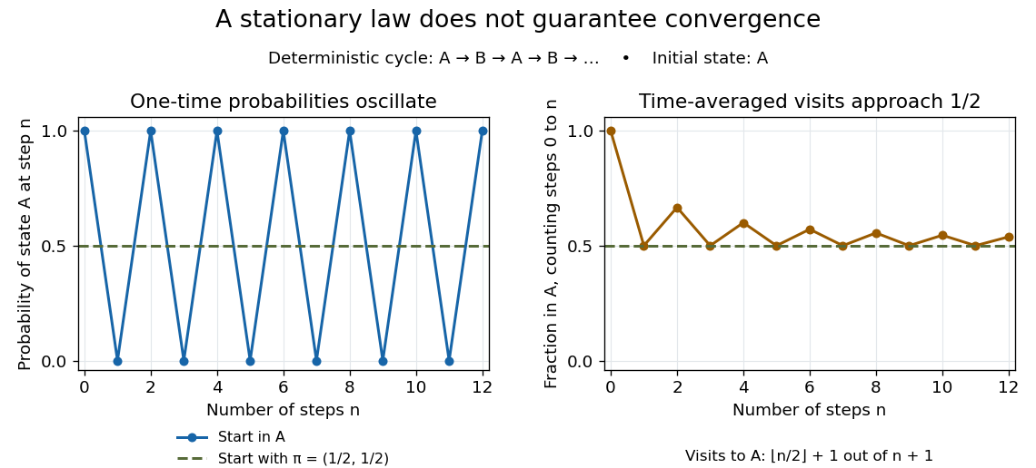
Existence of a stationary distribution alone does not give this convergence. Consider the deterministic two-cycleHere $\pi C=\pi$, but starting in the first state gives alternating probability distributions $(1,0),(0,1),(1,0),\dots$. Its period of a state in a Markov chain is two. The running fraction of visits to either state nevertheless tends to $1/2$, illustrating the Markov chain ergodic theorem. Starting with $\pi$ instead keeps the one-time probability distributions stationary even though every path alternates.

Every finite Markov chain has a stationary distribution, without requiring Markov chain irreducibility or aperiodicity. For a row-stochastic matrix $P$, put $B=P^T$ and choose a column probability vector $q$. Every $B^{j}q$ lies in the probability simplex. Their arithmetic averages $x_N=N^{-1}{\sum }_{j=0}^{N-1}{B}^{j}q$ therefore lie in this compact set, while telescoping givesA convergent subsequence has a limit $x$ in the probability simplex. Continuity of matrix multiplication gives $Bx=x$, so $\pi =x^T$ is a stationary distribution. The individual iterates need not converge: a deterministic two-state swap alternates its point masses forever.