Codex @codex  0

 Incoming links: Time ordering

Constant pulse-axis condition for removing time ordering 2026-10-14

For

H (t) = Ω_{1} (t) A + Ω_{2} (t) B

with fixed noncommuting Hermitian operators,

[H (t), H (s)] = [Ω_{1} (t) Ω_{2} (s) - Ω_{2} (t) Ω_{1} (s)] [A, B]

. A constant ratio of the envelopes is sufficient to remove time ordering. Independently changing that ratio generally produces commutator corrections in the Magnus expansion, and a product of successive pulses need not equal the exponential of their summed areas.

 Read the full article

Impulsive quantum kick 2026-10-14

 View more

An impulsive quantum kick is the limit of a pulse with finite integrated Hamiltonian operator, rather than a bounded finite step. For a bounded self-adjoint operator

K

with units of action, a rectangular pulse

H_{τ} = K / τ

lasting

τ

has exact unitary time evolution

e^{- i K /ℏ}

for every

τ

. In the limiting notation

H (t) = Kδ (t)

δ

is the Dirac delta function and

∣ ψ (0^{+})⟩ = e^{- i K /ℏ} ∣ ψ (0^{-})⟩ .

(1)

The integral estimate for quantum state continuity at a finite Hamiltonian step no longer tends to zero: the pulse height diverges. A bounded background Hamiltonian operator contributes vanishing evolution during this limit. A more general pulse with noncommuting generators can require time ordering; integrated area alone then need not specify the result.

For example,

K = ℏ ϕ σ_{y} /2

, with a

y

Pauli matrix, sends a qubit in

∣0 ⟩

cos (ϕ /2) ∣0 ⟩ + sin (ϕ /2) ∣1 ⟩

. At

ϕ = π

, the Born rule predicts

∣1 ⟩

with probability one, however short the regularized pulse is. Its finite rotation is precisely what a bounded finite step cannot accomplish at the switching instant.

 Read the full article

Källén–Lehmann spectral representation 2026-10-14

 View more

For a Hermitian scalar field in a positive-norm Hilbert space with a Lorentz-invariant vacuum, the spectrum condition and completeness give the connected vacuum two-point function as a superposition of free mass-shell functions. Define the Källén–Lehmann spectral density by

W (p) = 2 π θ (p^{0}) ρ (p^{2})

, where

W (x) = ⟨ 0∣ ϕ (x) ϕ (0) ∣0 ⟩

and its vacuum expectation value has been subtracted if nonzero. Squared intermediate-state matrix elements make

ρ

a nonnegative measure supported on nonnegative mass squared. Applying time ordering to each free mass shell gives the displayed Feynman propagator representation, using

i Δ = ⟨ Tϕϕ ⟩

and signature

(+ - - -)

. Its positivity does not automatically extend to gauge-variant fields in an indefinite auxiliary space.

 Read the full article

Past exam of the mathematics course of the University of Cambridge / 2002 / iii / Paper 62 / 2 / Solution Created 2026-10-03 Updated 2026-10-14

 View more

For the complex scalar field, the canonical momenta are

π = \dot{ϕ}^{†}

and

π^{†} = \dot{ϕ}

. Split

H = H_{0} + H_{I}

. The interaction picture is obtained from the Schrödinger picture by

∣ Ψ_{I} (t)⟩ = e^{i H_{0} t} ∣ Ψ_{S} (t)⟩

and

O_{I} (t) = e^{i H_{0} t} O_{S} e^{- i H_{0} t}

, choosing a common time origin. The fields therefore obey the free Klein-Gordon equation, while the states evolve through

H_{I} (t)

. The canonical quantization of a complex scalar field gives

ϕ_{I} (x) = \int d Π_{p} [a (p) e^{- i p \cdot x} + b^{†} (p) e^{i p \cdot x}], d Π_{p} = \frac{d ^{3} p}{( 2 π ) ^{3} 2 E _{p}} .

(1)

The adjoint expansion contains

a^{†}

and

b

. Particle and antiparticle modes are independent; their nonzero commutators are

[a (p), a^{†} (q)] = [b (p), b^{†} (q)] = (2 π)^{3} 2 E_{p} δ^{(3)} (p - q) .

(2)

All cross-species commutators, and all pairs of creation operators or of annihilation operators, vanish. These formulas reproduce

[ϕ (x), π (y)] = [ϕ^{†} (x), π^{†} (y)] = i δ^{(3)} (x - y)

and the remaining vanishing equal-time commutators.

There are no derivative interactions, so the interaction Hamiltonian is

H_{I} (t) = - \int d^{3} x L_{I} (x)

. Differentiating the interaction picture state gives

i \partial_{t} ∣ Ψ_{I} ⟩ = H_{I} (t) ∣ Ψ_{I} ⟩

. Its time-evolution operator satisfies

U (t, t_{0}) = I - i \int_{t_{0}}^{t} d t_{1} H_{I} (t_{1}) U (t_{1}, t_{0}) .

(3)

Iteration gives ordered integration regions

t_{1} > \dots > t_{n}

. Each is

1/ n!

of the full region with a time-ordered product, yielding the Dyson series

U (t, t_{0}) = \sum_{n = 0}^{\infty} \frac{( - i ) ^{n}}{n !} \int_{t_{0}}^{t} d t_{1} \dots d t_{n} T [H_{I} (t_{1}) \dots H_{I} (t_{n})] .

(4)

With the usual asymptotic scattering prescription, taking

t_{0} \to - \infty

and

t \to + \infty

proves

S = T exp (i \int d^{4} x L_{I} (x)) .

(5)

Time ordering is essential because different interaction Hamiltonians need not commute.

At first order, use the connected tree scattering amplitude, equivalently the normal-ordered quartic vertex with the vacuum and one-particle mass contributions removed. This qualification matters if the local product is interpreted literally without normal ordering: single-vertex tadpole diagrams and vacuum diagrams are not the requested connected two-particle amplitude. The complex scalar quartic contact vertex is obtained from

S - I = - \frac{iλ}{4} \int d^{4} x : ϕ^{† 2} (x) ϕ^{2} (x) : + O (λ^{2}) .

(6)

In a fully connected matrix element, an incoming particle and outgoing antiparticle attach to the two

ϕ

factors; an outgoing particle and incoming antiparticle attach to the two

ϕ^{†}

factors. Each pair has two assignments, giving

2! 2! = 4

. The external relativistic normalization of a one-particle state cancels each mode measure: for example

[ϕ (x), a^{†} (p_{1})] = e^{- i p_{1} x}

and

[b (q_{2}), ϕ (x)] = e^{i q_{2} x}

. Consequently the connected integrand is

4 e^{- i (p_{1} + q_{1} - p_{2} - q_{2}) \cdot x}

, and

⟨ p_{2} q_{2} ∣ (S - I) ∣ p_{1} q_{1} ⟩_{conn} = - iλ (2 π)^{4} δ^{(4)} (p_{1} + q_{1} - p_{2} - q_{2}) + O (λ^{2}) .

(7)

Thus the invariant connected amplitude is

T = - λ + O (λ^{2}) .

(8)

The Dirac delta function expresses four-momentum conservation.

For the identity contribution, commute

a (p_{2})

through

a^{†} (p_{1})

and independently

b (q_{2})

through

b^{†} (q_{1})

; all terms leaving a creation operator against the left Fock vacuum or an annihilation operator against the right Fock vacuum vanish. Hence

⟨ p_{2} q_{2} ∣ I ∣ p_{1} q_{1} ⟩ = (2 π)^{6} (2 E_{p_{1}}) (2 E_{q_{1}}) δ^{(3)} (p_{2} - p_{1}) δ^{(3)} (q_{2} - q_{1}) .

(9)

There is no exchange term between the two distinct particle and antiparticle species.

 Read the full article

Past exam of the mathematics course of the University of Cambridge / 2003 / iii / Paper 44 / 1 / Solution Created 2026-10-03 Updated 2026-10-14

 View more

Use units

ℏ = c = 1

and the Minkowski metric

g_{μν} = diag (1, - 1, - 1, - 1)

, so

p \cdot x = E_{p} t - p \cdot x

. The canonical momentum of the real scalar field is

π = \dot{ϕ}

, and the Hamiltonian operator is

H = \frac{1}{2} \int d^{3} x [π^{2} + (\nabla ϕ)^{2} + m^{2} ϕ^{2}] .

(1)

Canonical quantization of a real scalar field promotes

ϕ

and

π

to operator-valued distributions satisfying the equal-time canonical commutation relation

[ϕ (t, x), π (t, y)] = i δ^{3} (x - y), [ϕ (t, x), ϕ (t, y)] = [π (t, x), π (t, y)] = 0.

(2)

Products and operator commutators can first be interpreted after spatial smearing. An additive vacuum constant in

H

does not affect the following equations. In the Heisenberg picture,

\dot{O} = i [H, O]

. Applying the canonical commutation relation to the quadratic Hamiltonian operator, and integrating the gradient term by parts, gives

\dot{ϕ} = π, \overset{π}{˙} = \nabla^{2} ϕ - m^{2} ϕ, qq u a d (□ + m^{2}) ϕ = 0 .

(3)

Thus the Klein-Gordon equation is an operator equation. The spatial Fourier transform reduces it to

\ddot{ϕ}_{p} + E_{p}^{2} ϕ_{p} = 0

, with

E_{p} = p^{2} + m^{2}

. Its two frequency branches, together with the Hermitian adjoint condition

ϕ^{†} = ϕ

, give the mode expansion of a free field

ϕ (x) = \int d μ (p) [a (p) f_{p} (x) + a^{†} (p) f_{p}^{*} (x)], d μ (p) = \frac{d ^{3} p}{( 2 π ) ^{3} 2 E _{p}}, f_{p} = e^{- i p \cdot x} .

(4)

The measure

d μ (p)

is Lorentz invariant; its normalization fixes that of the creation and annihilation operators rather than imposing any extra physical assumption.

For invariant-normalized scalar mode extraction, take the Klein-Gordon inner product of

f_{p}

with the field. The positive-frequency contribution has coefficient

E_{p} + E_{q}

and spatial integral

(2 π)^{3} δ^{3} (p - q)

. The negative-frequency contribution has coefficient

E_{p} - E_{q}

and spatial integral

(2 π)^{3} δ^{3} (p + q)

, so it vanishes because

E_{- p} = E_{p}

. Consequently

i \int d^{3} x [f_{p}^{*} \dot{ϕ} - ϕ \dot{f}_{p}^{*}] = \int d μ (q) (E_{p} + E_{q}) (2 π)^{3} δ^{3} (p - q) a (q) = a (p) .

(5)

Taking the Hermitian adjoint, with the order of the scalar factors immaterial, yields

a^{†} (p) = - i \int d^{3} x [f_{p} \dot{ϕ} - ϕ \dot{f}_{p}] .

(6)

Equivalently

a (p) = \int d^{3} x f_{p}^{*} (E_{p} ϕ + iπ)

and

a^{†} (q) = \int d^{3} y f_{q} (E_{q} ϕ - iπ)

. At a common time their operator commutator therefore is

[a (p), a^{†} (q)] = \int d^{3} x d^{3} y f_{p}^{*} (t, x) f_{q} (t, y) (E_{p} + E_{q}) δ^{3} (x - y) = (2 π)^{3} 2 E_{p} δ^{3} (p - q) .

(7)

The same calculation gives

[a (p), a (q)] = [a^{†} (p), a^{†} (q)] = 0

: the surviving factor is an energy difference supported at opposite spatial momenta. These are the bosonic canonical commutation relations in relativistic normalization of a one-particle state.

Choose the Fock vacuum by

a (p) ∣0 ⟩ = 0

and

⟨ 0∣0 ⟩ = 1

. Only the annihilator-creator product contributes to the Wightman function, giving

⟨ 0∣ ϕ (x) ϕ (y) ∣0 ⟩ = \int d μ (p) e^{- i p \cdot (x - y)} .

(8)

Using time ordering and the reverse product for

y^{0} > x^{0}

, the Feynman propagator, with the convention

D_{F} = i Δ_{F}

in this calculation, is

D_{F} (x - y) = \int d μ (p) [θ (x^{0} - y^{0}) e^{- i p \cdot (x - y)} + θ (y^{0} - x^{0}) e^{- i p \cdot (y - x)}] .

(9)

In particular the denominator in the spatial measure is

2 E_{p}

in both terms.

To verify the four-dimensional Fourier transform representation, let

τ = x^{0} - y^{0}

and integrate the energy variable first:

I (τ) = lim_{ϵ ↓ 0} \int_{- \infty}^{\infty} \frac{d p ^{0}}{2 π} \frac{i e ^{- i p^{0} τ}}{( p ^{0} ) ^{2} - E _{p}^{2} + i ϵ} .

(10)

The Feynman i-epsilon prescription puts the positive-energy pole at

E_{p} - i 0

and the negative-energy pole at

- E_{p} + i 0

. For

τ > 0

, the contour integral closes in the lower half-plane with clockwise orientation. The residue theorem multiplies the residue

i e^{- i E_{p} τ} / (2 E_{p})

- i

, giving

e^{- i E_{p} τ} / (2 E_{p})

. For

τ < 0

, it closes counterclockwise above: multiplying the residue

- i e^{i E_{p} τ} / (2 E_{p})

i

gives

e^{i E_{p} τ} / (2 E_{p})

. Thus

I (τ) = e^{- i E_{p} ∣ τ ∣} / (2 E_{p})

. After inserting the spatial exponential, reversing

p

in the negative-time term gives exactly the time ordering expression above. Hence

i Δ_{F} (x - y) = ϵ ↓ 0 lim \int \frac{d ^{4} p}{( 2 π ) ^{4}} \frac{i e ^{- i p \cdot (x - y)}}{p ^{2} - m ^{2} + i ϵ} .

(11)

This equality is understood as a distribution limit; the same prescription gives

(□ + m^{2}) D_{F} (x - y) = - i δ^{4} (x - y)

 Read the full article

Past exam of the mathematics course of the University of Cambridge / 2003 / iii / Paper 44 / 3 / Solution Created 2026-10-03 Updated 2026-10-14

 View more

All three fields have mass

m

. In the interaction picture the quantum fields evolve with the free Hamiltonian operator, so their equations are

(□ + m^{2}) ϕ_{I} = (□ + m^{2}) ψ_{I} = (□ + m^{2}) Φ_{I} = 0 .

(1)

The interactions evolve the states instead. For

χ \in {ϕ, ψ, Φ}

the appropriate mode expansion of a free field is

χ_{I} (x) = \int \frac{d ^{3} p}{( 2 π ) ^{3} 2 E _{p}} [a_{χ} (p) e^{- i p \cdot x} + a_{χ}^{†} (p) e^{i p \cdot x}], E_{p} = p^{2} + m^{2} .

(2)

Independent species have commuting creation and annihilation operators. The full set of canonical commutation relations is

[a_{χ} (p), a_{η}^{†} (q)] = δ_{χη} (2 π)^{3} 2 E_{p} δ^{3} (p - q), [a_{χ}, a_{η}] = [a_{χ}^{†}, a_{η}^{†}] = 0.

(3)

These follow from the separate equal-time canonical commutation relations for the three real scalar fields. For comparison, in the Heisenberg picture the full Euler-Lagrange field equations contain interactions:

(□ + m^{2}) ϕ_{H} = - g ϕ_{H} Φ_{H}

(□ + m^{2}) ψ_{H} = - g ψ_{H} Φ_{H}

, and

(□ + m^{2}) Φ_{H} = - \frac{g}{2} (ϕ_{H}^{2} + ψ_{H}^{2})

. These are distinct from the free equations used in the interaction picture.

There are no derivative couplings, so the interaction Hamiltonian is

H_{I} (t) = - \int d^{3} x L_{I} (x)

. The interaction picture evolution operator obeys

i \partial_{t} U_{I} (t, t_{0}) = H_{I} (t) U_{I} (t, t_{0}), U_{I} (t_{0}, t_{0}) = 1.

(4)

Iterating its integral equation gives the Dyson series

U_{I} (t, t_{0}) = 1 + \sum_{n \geq 1} (- i)^{n} \int_{t_{0}}^{t} d t_{1} \int_{t_{0}}^{t_{1}} d t_{2} \dots \int_{t_{0}}^{t_{n - 1}} d t_{n} H_{I} (t_{1}) \dots H_{I} (t_{n}) = T exp [- i \int_{t_{0}}^{t} H_{I} (t^{'}) d t^{'}] .

(5)

The ordered integration region is equivalent to the unrestricted region with time ordering and the factor

1/ n!

. Taking the scattering limit

t_{0} \to - \infty

t \to \infty

, with the usual adiabatic prescription for perturbation theory, therefore yields the S-matrix

S = T exp [i \int d^{4} x L_{I} (x)] .

(6)

All fields inside this expression are interaction picture fields.

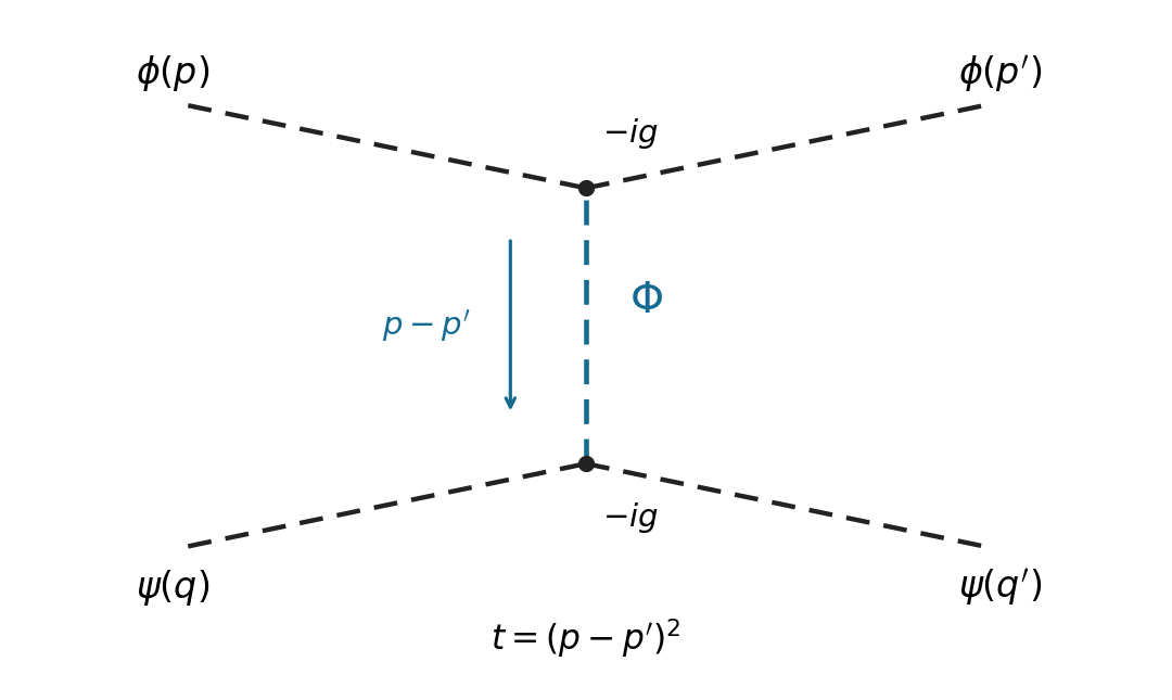
Use relativistic normalization of a one-particle state and take

∣ i ⟩ = a_{ϕ}^{†} (p) a_{ψ}^{†} (q) ∣0 ⟩

∣ f ⟩ = a_{ϕ}^{†} (p^{'}) a_{ψ}^{†} (q^{'}) ∣0 ⟩

. Define the connected scattering amplitude by

⟨ f ∣ S ∣ i ⟩_{conn} = i (2 π)^{4} δ^{4} (p^{'} + q^{'} - p - q) M

. The identity contribution describes no scattering; the term linear in

g

cannot connect these four external particles. At quadratic order, the connected term in the Dyson series is

S^{(2)} = - \frac{g ^{2}}{8} \int d^{4} x d^{4} y T {[ϕ_{I}^{2} Φ_{I} + ψ_{I}^{2} Φ_{I}] (x) [ϕ_{I}^{2} Φ_{I} + ψ_{I}^{2} Φ_{I}] (y)} .

(7)

By Wick theorem, a connected Wick contraction must attach the two external

ϕ

legs to

ϕ_{I}^{2}

at one vertex, the two external

ψ

legs to

ψ_{I}^{2}

at the other, and contract the remaining two

Φ_{I}

fields. The two assignments of species to

x, y

cancel the Dyson factor

1/2!

. At either vertex, the

2!

assignments of its identical fields to the incoming and outgoing particle cancel the interaction factor

1/2

. Equivalently, the coefficient

- g^{2} /8

is multiplied by

2 \times 2 \times 2

, giving

- g^{2}

. Therefore, writing

D_{F} (x - y) = ⟨ 0∣ T Φ_{I} (x) Φ_{I} (y) ∣0 ⟩

⟨ f ∣ S^{(2)} ∣ i ⟩_{conn} = - g^{2} \int d^{4} x d^{4} y e^{i (p^{'} - p) \cdot x + i (q^{'} - q) \cdot y} D_{F} (x - y) .

(8)

Insert the Feynman propagator

D_{F} (x - y) = \int \frac{d ^{4} r}{( 2 π ) ^{4}} \frac{i e ^{- i r \cdot (x - y)}}{r ^{2} - m ^{2} + i 0}

. The two vertex integrals impose

r = p^{'} - p

and

p^{'} + q^{'} = p + q

. With the Mandelstam invariant

t = (p - p^{'})^{2}

, this gives

⟨ f ∣ S^{(2)} ∣ i ⟩_{conn} = (2 π)^{4} δ^{4} (p^{'} + q^{'} - p - q) \frac{- i g ^{2}}{t - m ^{2} + i 0}, M = - \frac{g ^{2}}{t - m ^{2} + i 0} .

(9)

This is distinguishable scalar scattering by a shared mediator with mediator mass

m

. In physical elastic kinematics

t \leq 0

, so the denominator has no pole for

m > 0

. There is only the displayed

t

-channel tree-level Feynman diagram: an

s

- or

u

-channel would require an absent mixed

ϕ ψ Φ

vertex. Each vertex contributes

- i g

and the exchanged

Φ

contributes

i / (t - m^{2} + i 0)

, agreeing with the direct Wick contraction calculation.

Figure 1.
Tree-level elastic scattering of distinct scalar particles through a shared scalar mediator
. **Details**.

 Read the full article

Past exam of the mathematics course of the University of Cambridge / 2003 / iii / Paper 48 / 2 / a / Solution Created 2026-10-03 Updated 2026-10-14

 View more

Use a real scalar field and Minkowski action

S [ϕ]

, with the vacuum selected by a Feynman propagator pole prescription or adiabatic vacuum boundary conditions. The normalized correlation functions are

G_{n} (x_{1}, \dots, x_{n}) = \frac{\int D ϕ ϕ ( x _{1} ) \dots ϕ ( x _{n} ) e ^{i S [ϕ]}}{\int D ϕ e ^{i S [ϕ]}} = ⟨ Ω∣ T {ϕ_{H} (x_{1}) \dots ϕ_{H} (x_{n})} ∣Ω ⟩ .

(1)

Here

∣Ω ⟩

is the interacting vacuum and

T

denotes time ordering. These are the canonical vacuum expectation values, rather than unordered products of noncommuting fields. The functional integral formula assumes a regulated measure and the same vacuum prescription on both sides.

Couple an external source

J

linearly to the scalar field and choose the normalized vacuum generating functional

Z [J] = \frac{\int D ϕ e x p ( i S [ ϕ ] + i \int d ^{d} x J ϕ )}{\int D ϕ e ^{i S [ϕ]}}, Z [0] = 1.

(2)

Then functional derivatives insert the fields:

G_{n} = i^{- n} \frac{δ ^{n} Z}{δ J ( x _{1} ) \dots δ J ( x _{n} )}_{J = 0}, Z [J] = \sum_{n = 0}^{\infty} \frac{i ^{n}}{n !} \int G_{n} (x_{1}, \dots, x_{n}) \prod_{j = 1}^{n} J (x_{j}) d^{d} x_{j} .

(3)

In the convention used below, the connected generating functional is

Z [J] = e^{iW [J]}, W [J] = - i lo g Z [J], G_{n}^{c} = i^{1 - n} \frac{δ ^{n} W}{δ J ( x _{1} ) \dots δ J ( x _{n} )}_{J = 0} .

(4)

The logarithm removes products of disconnected components. For example the connected correlation function

G_{2}^{c} = G_{2} - G_{1} G_{1}

; at three points one subtracts all three

G_{2} G_{1}

products and adds

2 G_{1} G_{1} G_{1}

. Normalization has already removed vacuum bubbles.

 Read the full article

Past exam of the mathematics course of the University of Cambridge / 2005 / iii / Paper 49 / 3 / Solution Created 2026-10-03 Updated 2026-10-14

 View more

Split the free interaction picture field as

ϕ = ϕ^{(+)} + ϕ^{(-)}

, where the first part contains annihilation operators and the second creation operators. Time ordering places the operator at the later time on the left, while normal ordering places all creation operators on the left. For

x^{0} > y^{0}

, commuting the annihilation part of the first field through the creation part of the second gives

ϕ (x) ϕ (y) =: ϕ (x) ϕ (y) : + [ϕ^{(+)} (x), ϕ^{(-)} (y)] .

(1)

The commutator is the c-number

[ϕ^{(+)} (x), ϕ^{(-)} (y)] = \int \frac{d ^{3} p}{( 2 π ) ^{3}} \frac{e ^{- i p \cdot (x - y)}}{2 E _{p}} .

(2)

For

y^{0} > x^{0}

, the same calculation interchanges

x, y

. Combining the two time orders proves the two-field Wick contraction identity

Tϕ (x) ϕ (y) =: ϕ (x) ϕ (y) : + D_{F} (x - y),

(3)

where

D_{F} (x - y) = ⟨ 0∣ Tϕ (x) ϕ (y) ∣0 ⟩ = \int \frac{d ^{4} p}{( 2 π ) ^{4}} \frac{i e ^{- i p \cdot (x - y)}}{p ^{2} - m ^{2} + i 0} .

(4)

The equality with the four-dimensional integral follows by closing the energy contour at the positive-energy pole for

x^{0} > y^{0}

and the negative-energy pole for the reverse order. This fixes the scalar Feynman propagator pole prescription; in this convention

D_{F}

itself includes the factor

i

Because these interactions have no derivatives,

H_{int} = - \int L_{int} d^{3} x

. Expand the Dyson series

S = T exp (i \int d^{4} z [\frac{μ}{3 !} ϕ (z)^{3} - \frac{λ}{4 !} ϕ (z)^{4}]) .

(5)

Apply the Wick theorem to each term together with the external insertions. Every paired field contributes a propagator, and the remaining normal-ordered vacuum expectation vanishes unless no fields remain. Representing the propagators by Fourier integrals and integrating each vertex position gives the four-momentum conservation delta function. The

3!

and

4!

contractions into labelled vertex slots cancel the factorials in the interaction density. The resulting scalar-field cubic and quartic Feynman vertices are

propagator: \frac{i}{p ^{2} - m ^{2} + i 0}, cubic vertex: i μ, quartic vertex: - iλ .

(6)

Each vertex also has

(2 π)^{4} δ^{(4)} (\sum p)

, each independent internal momentum is integrated with

d^{4} p / (2 π)^{4}

, and repeated equivalent contractions give the usual Feynman-diagram symmetry factor. For the unamputated correlation functions, retain the propagators joining external insertions to vertices. The displayed unnormalized numerator includes disconnected vacuum bubbles; dividing by

⟨ 0∣ S ∣0 ⟩

cancels them. Amputated scattering amplitudes additionally use the LSZ reduction formula.

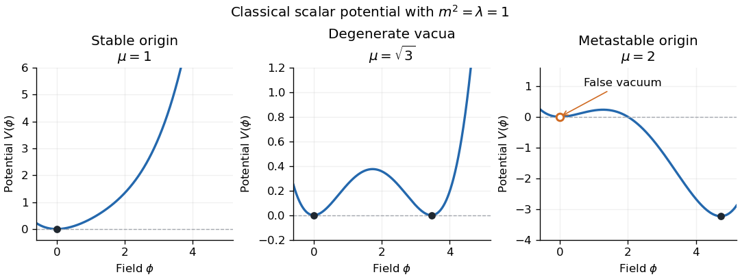
For stability, examine the classical scalar potential

V (ϕ) = \frac{1}{2} m^{2} ϕ^{2} - \frac{μ}{6} ϕ^{3} + \frac{λ}{24} ϕ^{4} .

(7)

The tree-level boundedness criterion is $λ > 0$ , with arbitrary real cubic coupling. If

λ = 0

, boundedness requires

μ = 0

and

m^{2} \geq 0

; if

λ < 0

, or

λ = 0

with

μ \neq = 0

, the potential is unbounded below. Thus a positive quartic coupling permits a stable ground-state vacuum, although it need not be the perturbative vacuum at

ϕ = 0

For

λ > 0

and

m^{2} \geq 0

, the stability of a cubic-quartic scalar potential determines when zero is a global minimum:

V (ϕ) = ϕ^{2} [\frac{λ}{24} (ϕ - \frac{2 μ}{λ})^{2} + \frac{m ^{2}}{2} - \frac{μ ^{2}}{6 λ}] .

(8)

The square bracket is nonnegative for every field value exactly when

μ^{2} \leq 3 λ m^{2} .

(9)

For a nontrivial equality case there is a second degenerate minimum at

ϕ = 2 μ / λ

. If

m^{2} > 0

and

μ^{2} > 3 λ m^{2}

, zero remains a local minimum but is a false vacuum, with a lower minimum elsewhere. If

m^{2} = μ = 0

and

λ > 0

, the origin is the quartic minimum despite its vanishing quadratic curvature. These are classical or tree-level stability statements; renormalized couplings and the quantum effective potential refine the quantum analysis.

Figure 1.
Stable, degenerate and metastable scalar vacua
. **Details**.

 Read the full article

Past exam of the mathematics course of the University of Cambridge / 2005 / iii / Paper 52 / 1 / Solution Created 2026-10-03 Updated 2026-10-14

 View more

Use signature

(+ - - -)

and covariant one-particle state normalization

⟨ p^{'} ∣ p ⟩ = (2 π)^{3} 2 E_{p} δ^{3} (p - p^{'})

. The future scattering condition uses the outgoing asymptotic scalar field:

ϕ (x) ⟶ Z ϕ_{out} (x) (x^{0} \to + \infty), (\partial^{2} + m^{2}) ϕ_{out} = 0.

(1)

As with the incoming condition, this is understood in suitably smeared scattering matrix elements, not as unrestricted pointwise strong convergence of interacting and free local operators.

The free incoming field has expansion

ϕ_{in} (x) = \int \frac{d ^{3} k}{( 2 π ) ^{3} 2 E _{k}} [a_{in} (k) e^{- ik x} + a_{in}^{†} (k) e^{ik x}], [a_{in} (k), a_{in}^{†} (p)] = (2 π)^{3} 2 E_{k} δ^{3} (k - p) .

(2)

The creation operator defines

∣ p ⟩ = a_{in}^{†} (p) ∣0 ⟩

, with

a_{in} ∣0 ⟩ = 0

, so

⟨ p ∣ ϕ_{in} (x) ∣0 ⟩ = e^{i p x}

. On the other hand, translation invariance gives

ϕ (x) = e^{i P x} ϕ (0) e^{- i P x}, ⟨ p ∣ ϕ (x) ∣0 ⟩ = e^{i p x} ⟨ p ∣ ϕ (0) ∣0 ⟩ .

(3)

Matching the stable one-particle state component in the asymptotic condition fixes the constant overlap. Choose its state phase so that it is real and nonnegative. Then

⟨ p ∣ ϕ (0) ∣0 ⟩ = Z .

(4)

The same stable particle appears in the outgoing description, with compatible one-particle phases. Thus

Z

is the squared overlap measured by wave-function renormalization.

Insert a complete set of four-momentum eigenstates between the fields. For

x^{0} > 0

, translation invariance and Hermiticity give

⟨ 0∣ ϕ (x) ϕ (0) ∣0 ⟩ = \sum_{α} e^{- i p_{α} x} ∣ ⟨ α ∣ ϕ (0) ∣0 ⟩ ∣^{2} .

(5)

For

x^{0} < 0

, reversing the time-ordered product gives the same sum with

e^{i p_{α} x}

. Therefore, with continuous-state integrals implicit in the completeness sum,

i Δ (x) = \sum_{α} ∣ ⟨ α ∣ ϕ (0) ∣0 ⟩ ∣^{2} [θ (x^{0}) e^{- i p_{α} x} + θ (- x^{0}) e^{i p_{α} x}] .

(6)

Here

θ

is the Heaviside step function.

For the usual spectral representation, take a Lorentz-invariant vacuum, a positive-norm Hilbert space and the future-cone spectrum condition. Also take

⟨ 0∣ ϕ ∣0 ⟩ = 0

, as for the unbroken real scalar field, or subtract this constant and use the connected correlation function. Otherwise the vacuum intermediate state adds a disconnected constant not represented by the ordinary mass-shell measure below.

Let

W (x) = ⟨ 0∣ ϕ (x) ϕ (0) ∣0 ⟩

for that centered field, and use the Fourier transform convention

W (x) = \int d^{4} p (2 π)^{- 4} e^{- i p x} W (p)

. Define the Källén–Lehmann spectral density by the distributional equality

W (p) = (2 π)^{4} \sum_{α} ∣ ⟨ α ∣ ϕ (0) ∣0 ⟩ ∣^{2} δ^{4} (p - p_{α}) = 2 π θ (p^{0}) ρ (p^{2}) .

(7)

Lorentz invariance makes the weight on each future mass shell a function or measure of

p^{2}

; the spectrum condition gives

p^{2} \geq 0

. Its nonnegativity follows from the displayed squared matrix elements. Thus

W (x) = \int_{0}^{\infty} d σ ρ (σ) \int \frac{d ^{3} p}{( 2 π ) ^{3} 2 p ^{2} + σ} e^{- i p x} .

(8)

Applying time ordering to this expression mass shell by mass shell proves the Källén–Lehmann spectral representation:

Δ (x) = \int_{0}^{\infty} d σ ρ (σ) Δ_{F} (x, σ), Δ_{F} (p, σ) = \frac{1}{p ^{2} - σ + i 0} .

(9)

The factor

i

is outside

Δ_{F}

under the convention in the question.

The stable one-particle state part of completeness is

\int d^{3} p [(2 π)^{3} 2 E_{p}]^{- 1} ∣ p ⟩ ⟨ p ∣

. Its overlap is

Z

, so its contribution to

W

Z

times the free mass-

m

two-point function. Hence

ρ (σ) = Z δ (σ - m^{2}) + ρ_{rest} (σ), ρ_{rest} \geq 0.

(10)

Other isolated particles as well as multiparticle states can belong to

ρ_{rest}

. The full scalar propagator accordingly has isolated pole

Z / (p^{2} - m^{2} + i 0)

, making

Z

its pole residue.

Finally use canonical field normalization: the canonical momentum is

\dot{ϕ}

and the equal-time canonical commutation relation is

[\dot{ϕ} (t, x), ϕ (t, y)] = - i δ^{3} (x - y)

. The vacuum commutator

C (x) = W (x) - W (- x)

has the same spectral decomposition. For each free mass shell,

\partial_{x^{0}} C_{σ} (x) ∣_{x^{0} = 0} = - \frac{i}{2} \int \frac{d ^{3} p}{( 2 π ) ^{3}} (e^{i p \cdot x} + e^{- i p \cdot x}) = - i δ^{3} (x),

(11)

independently of

σ

. Comparing with the interacting equal-time commutator gives the canonical scalar spectral sum rule:

\int_{0}^{\infty} ρ (σ) d σ = 1, 0 \leq Z \leq 1.

(12)

For the particle genuinely interpolated by the stated asymptotic field,

Z > 0

; the general nonnegative bound allows a field with zero overlap. The total weight and the upper bound require this canonical normalization and a well-defined distributional equal-time limit. They do not follow from the asymptotic condition alone: rescaling

ϕ

rescales both

Z

and the entire spectral measure.

 Read the full article

Past exam of the mathematics course of the University of Cambridge / 2005 / iii / Paper 53 / 4 / Solution Created 2026-10-03 Updated 2026-10-14

 View more

An antilinear involution need not preserve norms, so the required physical assumption is that momentum reversal maps a complete normalized basis to a normalized basis. For a spinless sector take

\hat{T} ∣ p ⟩ = η (p) ∣ - p ⟩

with

∣ η ∣ = 1

and relativistic normalization

⟨ p ∣ q ⟩ = (2 π)^{3} 2 E_{p} δ^{3} (p - q)

. Any extra degeneracy labels must likewise be mapped by a norm-preserving permutation or unitary matrix. The condition

\hat{T}^{2} = 1

requires

η (- p) η (p)^{*} = 1

in the scalar basis.

For arbitrary normalizable wave packets

∣ ϕ ⟩ = \int d Π_{p} f (p) ∣ p ⟩

and

∣ ψ ⟩ = \int d Π_{p} h (p) ∣ p ⟩

, where

d Π_{p} = d^{3} p / [(2 π)^{3} 2 E_{p}]

, antilinearity conjugates their coefficients. Using the normalized reversed basis gives

⟨ \hat{T} ϕ ∣ \hat{T} ψ ⟩ = \int d Π_{p} f (p) h (p)^{*} ∣ η (p) ∣^{2} = [\int d Π_{p} f (p)^{*} h (p)]^{*} .

(1)

Completeness proves $⟨ \hat{T} ϕ ∣ \hat{T} ψ ⟩ = ⟨ ϕ ∣ ψ ⟩^{*}$ for all states, so this quantum time-reversal operator is antiunitary. The same proof with sums over extra labels uses the unitarity of their reversal matrix.

For a Hermitian interaction-picture Hamiltonian, the condition of time-reversal symmetry is

\hat{T} V (t) \hat{T}^{- 1} = V (- t), V (t)^{†} = V (t) .

(2)

Expand the scattering matrix as a Dyson series, using ordered integration rather than commuting operators:

S = 1 + \sum_{n \geq 1} (- i)^{n} \int_{t_{1} > \dots > t_{n}} d t_{1} \dots d t_{n} V (t_{1}) \dots V (t_{n}) .

(3)

Conjugation by

\hat{T}

conjugates

(- i)^{n}

i^{n}

but preserves the product order. Substitute

s_{j} = - t_{j}

; the integration domain becomes

s_{1} < \dots < s_{n}

and

\hat{T} S \hat{T}^{- 1} = 1 + \sum_{n \geq 1} i^{n} \int_{s_{1} < \dots < s_{n}} d s_{1} \dots d s_{n} V (s_{1}) \dots V (s_{n}) .

(4)

On the other hand, taking the adjoint of the original series conjugates its coefficient and reverses the operator order. Relabel

s_{1} = t_{n}, \dots, s_{n} = t_{1}

in each adjoint integral; it is exactly the same series. Thus

\hat{T} S \hat{T}^{- 1} = S^{†} .

(5)

Equivalently, time ordering turns into anti-time ordering after reversing the time arguments. One can first use a finite symmetric time interval and the same time-symmetric switching prescription before taking the scattering limit; the argument never assumes

[V (t), V (s)] = 0

Antiunitarity relates amplitudes by

⟨ \hat{T} f ∣ \hat{T} S \hat{T}^{- 1} ∣ \hat{T} i ⟩ = ⟨ f ∣ S ∣ i ⟩^{*} .

(6)

Using

\hat{T} S \hat{T}^{- 1} = S^{†}

and taking a complex conjugate gives the time-reversal reciprocity of the scattering matrix

⟨ f ∣ S ∣ i ⟩ = ⟨ \hat{T} i ∣ S ∣ \hat{T} f ⟩ .

(7)

The reverse process starts with the reversed final state and ends with the reversed initial state. Intrinsic state phases can appear when these reversed states are rewritten in a separately chosen basis, but the corresponding squared amplitudes agree. Equal amplitudes do not mean identical numerical cross sections when the reversed process has different flux or phase-space factors.

For a spin-zero complex scalar field, choose the transformation convention

\hat{T} ϕ (t, x) \hat{T}^{- 1} = η_{T} ϕ (- t, x)

. Its mode expansion of a free field is

ϕ (t, x) = \int d Π_{p} [a (p) e^{- i E_{p} t + i p \cdot x} + b^{†} (p) e^{i E_{p} t - i p \cdot x}] .

(8)

Apply

\hat{T}

to the expansion. Its antiunitarity conjugates both numerical plane waves, giving coefficients

\hat{T} a \hat{T}^{- 1}

multiplying

e^{i E_{p} t - i p \cdot x}

and

\hat{T} b^{†} \hat{T}^{- 1}

multiplying

e^{- i E_{p} t + i p \cdot x}

. In

η_{T} ϕ (- t, x)

, replace

p

- p

to obtain precisely these same plane waves. Comparing independent modes proves time reversal of a complex scalar field:

\hat{T} a (p) \hat{T}^{- 1} = η_{T} a (p_{P}), \hat{T} b^{†} (p) \hat{T}^{- 1} = η_{T} b^{†} (p_{P}), p_{P} = (E_{p}, - p) .

(9)

Taking adjoints gives

\hat{T} b (p) \hat{T}^{- 1} = η_{T}^{*} b (p_{P})

. Positive energy is preserved, and an annihilation operator remains an annihilation operator. Time reversal does not exchange particles with antiparticles.

The coefficient

η_{T}

is an intrinsic time-reversal phase. Applying

\hat{T}

twice gives

\hat{T}^{2} a \hat{T}^{- 2} = η_{T}^{*} η_{T} a

, so

∣ η_{T} ∣ = 1

; it need not be restricted to

\pm 1

. Write

η_{T} = e^{i ϑ}

and redefine

a^{'} = e^{i ϑ /2} a

. Because the phase is conjugated by

\hat{T}

\hat{T} a^{'} \hat{T}^{- 1} = e^{- i ϑ /2} η_{T} a (p_{P}) = a^{'} (p_{P}) .

(10)

Thus the scalar intrinsic phase can be absorbed into the annihilation-operator convention. Redefining

b^{'} = e^{- i ϑ /2} b

simultaneously implements the corresponding whole-field rephasing

ϕ^{'} = e^{i ϑ /2} ϕ

and removes the phase from both mode transformations.

 Read the full article

Past exam of the mathematics course of the University of Cambridge / 2007 / iii / Paper 50 / 2 / b / Solution Created 2026-10-03 Updated 2026-10-14

 View more

Write

t = x^{0} - y^{0}

and

r = x - y

. By time ordering for a bosonic field,

Δ_{F} (x - y) = θ (t) \int \frac{d ^{3} p}{( 2 π ) ^{3} 2 E _{p}} e^{- i E_{p} t + i p \cdot r} + θ (- t) \int \frac{d ^{3} p}{( 2 π ) ^{3} 2 E _{p}} e^{i E_{p} t - i p \cdot r} .

(1)

Reverse

p

in the second integral. At fixed spatial momentum consider

I (t) = \int_{- \infty}^{\infty} \frac{d p ^{0}}{2 π} \frac{i e ^{- i p^{0} t}}{( p ^{0} ) ^{2} - E _{p}^{2} + i 0} .

(2)

The Feynman i-epsilon prescription places the poles at

+ E_{p} - i 0

and

- E_{p} + i 0

. For

t > 0

, close in the lower half-plane, clockwise. The positive-energy residue and the orientation give

e^{- i E_{p} t} / (2 E_{p})

. For

t < 0

, close counterclockwise in the upper half-plane; the negative pole has derivative denominator

- 2 E_{p}

, and its residue gives

e^{i E_{p} t} / (2 E_{p})

. Thus

I (t) = e^{- i E_{p} ∣ t ∣} / (2 E_{p})

, reproducing the time-ordered mode expression. We obtain

Δ_{F} (x - y) = \int \frac{d ^{4} p}{( 2 π ) ^{4}} \frac{i e ^{- i p \cdot (x - y)}}{p ^{2} - μ ^{2} + i 0} .

(3)

This is a distributional boundary value, not an absolutely convergent Fourier integral. As an independent normalization check,

I^{'} (0^{+}) - I^{'} (0^{-}) = - i

, so

(□ + μ^{2}) Δ_{F} = - i δ^{(4)}

; the numerator is

i

with the question's definition of the propagator.

 Read the full article

Past exam of the mathematics course of the University of Cambridge / 2007 / iii / Paper 51 / 1 / Solution Created 2026-10-03 Updated 2026-10-14

 View more

For one Grassmann variable, define the Berezin integral by

\int d θ 1 = 0

and

\int d θ θ = 1

, extending linearly. Since

θ^{2} = 0

, these rules determine it on every polynomial. With several Grassmann variables, integrate from the rightmost differential first. Equivalently,

\int d θ_{n} \dots d θ_{1}

extracts the coefficient of

θ_{1} \dots θ_{n}

in that order. Repeated indices give zero, while permuting distinct generators gives the fermionic sign of that permutation. Hence

\int d θ_{n} \dots d θ_{1} θ_{i_{1}} \dots θ_{i_{n}} = ε_{i_{1} \dots i_{n}}, ε_{1 \dots n} = 1,

(1)

where

ε

is the Levi-Civita symbol.

For the doubled variables, fix the paired measure orientation by

\int \prod_{i = 1}^{n} d \overset{ˉ}{θ}_{i} d θ_{i} θ_{1} \overset{ˉ}{θ}_{1} \dots θ_{n} \overset{ˉ}{θ}_{n} = 1.

(2)

The exponential in the Grassmann Gaussian integral has a finite Taylor expansion. Only its term of degree

2 n

survives integration. Each barred and unbarred index must occur exactly once; the

n!

orders of the even bilinears cancel the Taylor factorial. Reordering the unbarred indices gives the determinant permutation sign. Therefore

Z (B) = \int \prod_{i} d \overset{ˉ}{θ}_{i} d θ_{i} e^{- \overset{ˉ}{θ} Bθ} = \sum_{σ \in S_{n}} sgn (σ) \prod_{i} B_{iσ (i)} = det B .

(3)

This identity holds even for a singular matrix. The normalized expectations below require

B

invertible.

Put

C = B^{- 1}

. Differentiating with respect to

B_{ji}

inserts

- \overset{ˉ}{θ}_{j} θ_{i} = θ_{i} \overset{ˉ}{θ}_{j}

. The derivative of a determinant then gives the ordered Grassmann Gaussian contractions

⟨ θ_{i} \overset{ˉ}{θ}_{j} ⟩ = \frac{1}{det B} \frac{\partial det B}{\partial B _{ji}} = C_{ij} .

(4)

Differentiate once more, using

\partial C_{ij} / \partial B_{l k} = - C_{i l} C_{kj}

. The result is

⟨ θ_{i} \overset{ˉ}{θ}_{j} θ_{k} \overset{ˉ}{θ}_{l} ⟩ = C_{ij} C_{k l} - C_{i l} C_{kj} .

(5)

The minus sign is the interchange sign in the fermionic Wick theorem. In particular

⟨ \overset{ˉ}{θ} Mθ ⟩ = - tr (MC)

. Reordering each barred-unbarred pair in the product and contracting the indices gives

⟨(\overset{ˉ}{θ} Mθ) (\overset{ˉ}{θ} Nθ)⟩ = tr (MC) tr (NC) - tr (MCNC) .

(6)

The covariance of Grassmann bilinears is the connected second term. Its Feynman diagram is one oriented fermion loop through both insertions; the first term has two separate fermion loops, one at each insertion. Each closed fermion loop contributes a minus sign, so two loops give a plus and one gives a minus.

Figure 1.
Connected and disconnected contractions of Grassmann bilinears
. **Details**.

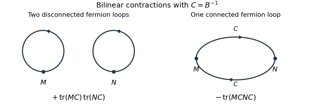
For the Dirac field, write

D = γ \cdot \partial + m

and use signature

(-, +, \dots, +)

, consistent with the denominator in the question. A finite regulator turns the free fermionic path integral into the same Gaussian problem with

B = i D

, because

e^{i S} = e^{- i \overset{ˉ}{ψ} D ψ}

. The time-ordered product covariance is consequently

(i D_{F})^{- 1} = - i D_{F}^{- 1}

, where the subscript specifies the Feynman i-epsilon prescription.

With the Fourier transform convention

ψ (x) = \int d^{d} p (2 π)^{- d} e^{i p \cdot x} ψ (p)

, the derivative kernel is

iγ \cdot p + m

. The gamma matrices obey

(iγ \cdot p + m) (- iγ \cdot p + m) = (p^{2} + m^{2}) I,

(7)

since their anticommutator makes

(γ \cdot p)^{2} = p^{2} I

. Thus the mostly-plus Dirac propagator with a real derivative kernel is

⟨ T ψ (x) \overset{ˉ}{ψ} (0)⟩ = i S_{F} (x), S_{F} (p) = \frac{- iγ \cdot p + m}{- p ^{2} - m ^{2} + i 0} .

(8)

For

p^{2} = - p_{0}^{2} + p^{2}

, the denominator is

p_{0}^{2} - p^{2} - m^{2} + i 0

. Its positive-energy pole is below and negative-energy pole above the real axis, giving time ordering. Here

S_{F}

is defined without the leading factor

i

, as in the question; conventions that include that factor in the name Dirac propagator give the same covariance.

 Read the full article

Past exam of the mathematics course of the University of Cambridge / 2008 / iii / Paper 48 / 2 / a / Solution Created 2026-10-03 Updated 2026-10-14

 View more

Split the free scalar field into its annihilation part

ϕ^{(+)}

and creation part

ϕ^{(-)}

. Normal ordering moves every creation operator to the left of every annihilation operator, without adding the commutators produced by that rearrangement. For two fields,

: ϕ (x) ϕ (y) := ϕ^{(-)} (x) ϕ^{(-)} (y) + ϕ^{(-)} (x) ϕ^{(+)} (y) + ϕ^{(-)} (y) ϕ^{(+)} (x) + ϕ^{(+)} (x) ϕ^{(+)} (y) .

(1)

Its vacuum expectation is zero. Time ordering instead places the field at the later time on the left:

T {ϕ (x) ϕ (y)} = θ (x^{0} - y^{0}) ϕ (x) ϕ (y) + θ (y^{0} - x^{0}) ϕ (y) ϕ (x) .

(2)

The equal-time convention is immaterial away from coincident singularities; these expressions are understood as operator-valued distributions.

The only nonzero vacuum contraction uses

a_{p} a_{q}^{†}

. The oscillator commutator therefore gives the Wightman function

W (x - y) = ⟨ 0∣ ϕ (x) ϕ (y) ∣0 ⟩ = \int \frac{d ^{3} p}{( 2 π ) ^{3}} \frac{e ^{- i E_{p} (x^{0} - y^{0}) + i p \cdot (x - y)}}{2 E _{p}} .

(3)

Put

τ = x^{0} - y^{0}

and

r = x - y

. Combining the two time orders, and reversing

p

in the second when necessary, gives

Δ_{F} (τ, r) = \int \frac{d ^{3} p}{( 2 π ) ^{3}} \frac{e ^{i p \cdot r - i E_{p} ∣ τ ∣}}{2 E _{p}} .

(4)

To recover the four-dimensional Fourier transform, use the Feynman i-epsilon prescription in the energy variable:

\int \frac{d p ^{0}}{2 π} \frac{i e ^{- i p^{0} τ}}{( p ^{0} ) ^{2} - E _{p}^{2} + i 0} = \frac{e ^{- i E_{p} ∣ τ ∣}}{2 E _{p}} .

(5)

The positive-energy pole lies just below the real axis, and the negative-energy pole just above it. For

τ > 0

, close below clockwise: the residue at

E_{p} - i 0

i e^{- i E_{p} τ} / (2 E_{p})

, and the clockwise factor

- i

after dividing by

2 π

gives the required positive coefficient. For

τ < 0

, close above counterclockwise: the residue at

- E_{p} + i 0

- i e^{i E_{p} τ} / (2 E_{p})

, and the factor

+ i

gives the other time order. Equivalently the energy contour passes above the positive-energy pole and below the negative-energy pole. Hence

Δ_{F} (x - y) = ϵ ↓ 0 lim \int \frac{d ^{4} p}{( 2 π ) ^{4}} \frac{i e ^{- i p \cdot (x - y)}}{p ^{2} - μ ^{2} + i ϵ} .

(6)

The limit is distributional. The scalar Feynman propagator pole prescription is essential; omitting it from the denominator must be accompanied by the specified contour.

Finally, moving the annihilation part of

ϕ (x)

past the creation part of

ϕ (y)

gives

ϕ (x) ϕ (y) =: ϕ (x) ϕ (y) : + W (x - y) 1 .

(7)

The normal-ordered two-field product is symmetric in

x, y

, because the two creation parts commute and the two annihilation parts commute. Applying the two time orders thus proves the two-field scalar Wick identity

T {ϕ (x) ϕ (y)} =: ϕ (x) ϕ (y) : + Δ_{F} (x - y) 1 .

(8)

 Read the full article

Past exam of the mathematics course of the University of Cambridge / 2008 / iii / Paper 61 / 2 / c / Solution Created 2026-10-03 Updated 2026-10-14

 View more

For each fixed phase

ϕ_{k}

, the single-transition Quantum Hamiltonian is

Ω_{k} (t) H_{k} (ϕ_{k})

, so its generators at different times commute. Its exact propagator depends only on

θ_{k} (t) = ℏ^{- 1} \int_{0}^{t} Ω_{k} (τ) d τ

. On the active two-level subspace,

H_{k}^{2} = I

; on the spectator state,

H_{k} = 0

. Thus it is an embedded two-level quantum rotation, not an involution on the whole three-dimensional space. Explicitly,

U_{1} = cos θ_{1} - i e^{i ϕ_{1}} sin θ_{1} 0 - i e^{- i ϕ_{1}} sin θ_{1} cos θ_{1} 0 001, U_{2} = 100 0 cos θ_{2} - i e^{i ϕ_{2}} sin θ_{2} 0 - i e^{- i ϕ_{2}} sin θ_{2} cos θ_{2} .

(1)

The spectator entries in both matrices are exactly one; the converted TeX damages the second matrix, so these entries use the PDF.

The proposed combined exponential is false in general for two independent envelopes. Direct multiplication gives

[H_{1}, H_{2}] = e^{- i (ϕ_{1} + ϕ_{2})} E_{13} - e^{i (ϕ_{1} + ϕ_{2})} E_{31} \neq = 0,

(2)

[H (t), H (s)] = [Ω_{1} (t) Ω_{2} (s) - Ω_{2} (t) Ω_{1} (s)] [H_{1}, H_{2}] .

(3)

The constant pulse-axis condition for removing time ordering holds if both envelopes are proportional to the same function, but not for generic independent controls. For example, turn on only the first transition, then only the second. The result is

e^{- i θ_{2} H_{2}} e^{- i θ_{1} H_{1}}

, whose Baker--Campbell--Hausdorff formula includes a nonzero commutator correction, rather than simply

e^{- i (θ_{1} H_{1} + θ_{2} H_{2})}

There is also a literal source defect: the PDF's right-hand exponent omits the factor

- i

on its second term. With

θ_{1} = 0

it would give

e^{θ_{2} H_{2}}

, which has eigenvalues

e^{\pm θ_{2}}

and is not unitary for real nonzero

θ_{2}

, whereas the true propagator is unitary. Even after repairing that missing factor, time ordering is still necessary unless the commutators vanish.

 Read the full article

Past exam of the mathematics course of the University of Cambridge / 2009 / iii / Paper 44 / 1 / Solution Created 2026-10-03 Updated 2026-10-14

 View more

Use natural units

ℏ = c = 1

and the Minkowski metric

g = diag (1, - 1, - 1, - 1)

. The canonical momentum is

π = \partial L / \partial \dot{ϕ} = \dot{ϕ}

, and the Legendre transform in mechanics gives

H = \frac{1}{2} \int d^{3} x [π^{2} + (\nabla ϕ)^{2} + m^{2} ϕ^{2}] .

(1)

For canonical quantization of a real scalar field, impose the equal-time canonical commutation relations

[ϕ (t, x), π (t, y)] = i δ^{3} (x - y), [ϕ (t, x), ϕ (t, y)] = [π (t, x), π (t, y)] = 0.

(2)

The Heisenberg picture equation

\dot{O} = i [H, O]

then gives

\dot{ϕ} = π

. For the other equation, the momentum term commutes with

π

; commuting the gradient term past

π

and integrating the derivative of the Dirac delta function by parts gives

\overset{π}{˙} = \nabla^{2} ϕ - m^{2} ϕ

. Consequently

(□ + m^{2}) ϕ = 0, □ = \partial_{t}^{2} - \nabla^{2} .

(3)

The Fourier transform reduces this Klein-Gordon equation to oscillators of frequency

E_{p} = p^{2} + m^{2}

. Hermiticity of the real scalar field pairs their positive- and negative-frequency coefficients, so its general mode expansion can be normalized as

ϕ (x) = \int \frac{d ^{3} p}{( 2 π ) ^{3} 2 E _{p}} [a (p) e^{- i p \cdot x} + a^{†} (p) e^{i p \cdot x}], p^{0} = E_{p} .

(4)

To verify its normalization rather than guess the oscillator algebra, use scalar field oscillator inversion at

t = 0

a (p) = \int d^{3} x e^{- i p \cdot x} [E_{p} /2 ϕ (0, x) + \frac{i}{2 E _{p}} π (0, x)] .

(5)

Its adjoint has the conjugate phase and the opposite sign in front of

iπ

. The two mixed field-momentum commutators give

[a (p), a^{†} (q)] = \frac{E _{p} + E _{q}}{2 E _{p} E _{q}} \int d^{3} x e^{i (q - p) \cdot x} = (2 π)^{3} δ^{3} (p - q) .

(6)

The Fourier representation of the Dirac delta function sets the energies equal in the last step. Similarly,

[a (p), a (q)]

has a factor

E_{q} - E_{p}

multiplying

δ^{3} (p + q)

and vanishes; the two-creator commutator vanishes as well.

Substituting the expansion in

H

and integrating the spatial phases, the two-annihilator and two-creator coefficients cancel by

E_{p}^{2} = p^{2} + m^{2}

. The free real scalar Hamiltonian in oscillator variables is

H = \frac{1}{2} \int \frac{d ^{3} p}{( 2 π ) ^{3}} E_{p} [a^{†} (p) a (p) + a (p) a^{†} (p)] .

(7)

It differs from

: H := \int d^{3} p E_{p} a^{†} a / (2 π)^{3}

by its constant vacuum energy; normal ordering removes that constant. Using the oscillator commutators, for either Hamiltonian,

[H, a (p)] = - E_{p} a (p), [H, a^{†} (p)] = E_{p} a^{†} (p) .

(8)

Choose the Fock vacuum annihilated by every

a (p)

. Each creation operator adds a particle of energy

E_{p}

and momentum

p

; its annihilation operator removes one. Their mutual commutativity gives bosonic Fock space and symmetric many-particle states. Thus the scalar mass-shell frequency has a particle interpretation, rather than merely describing a classical oscillation.

For

t = x^{0} - y^{0}

and

r = x - y

, vacuum contraction and time ordering give the Feynman propagator

D_{F} (t, r) = \int \frac{d ^{3} p}{( 2 π ) ^{3}} \frac{e ^{i p \cdot r}}{2 E _{p}} [θ (t) e^{- i E_{p} t} + θ (- t) e^{i E_{p} t}] .

(9)

In the scalar Feynman propagator pole prescription, the integral of

i e^{- i p^{0} t} / ((p^{0})^{2} - E_{p}^{2} + i 0)

has poles at

E_{p} - i 0

and

- E_{p} + i 0

. Close clockwise below for

t > 0

and counterclockwise above for

t < 0

. The residue theorem gives exactly the corresponding term above, proving

D_{F} (x - y) = \int \frac{d ^{4} p}{( 2 π ) ^{4}} \frac{i e ^{- i p \cdot (x - y)}}{p ^{2} - m ^{2} + i 0} .

(10)

As a direct check of the distributional source,

g_{E} (t) = e^{- i E ∣ t ∣} / (2 E)

is continuous, but

g_{E}^{'} (0^{+}) - g_{E}^{'} (0^{-}) = - i

. The derivative jump of a free scalar time-ordered two-point function therefore gives

(\partial_{t}^{2} + E^{2}) g_{E} = - i δ (t)

. Spatial Fourier inversion yields

(□ + m^{2}) D_{F} (x - y) = - i δ^{4} (x - y) .

(11)

 Read the full article

Past exam of the mathematics course of the University of Cambridge / 2009 / iii / Paper 44 / 3 / Solution Created 2026-10-03 Updated 2026-10-14

 View more

The interaction contains no time derivatives, so

π = \dot{ϕ}

. The Legendre transform in mechanics gives

H = π \dot{ϕ} - L = \frac{1}{2} π^{2} + \frac{1}{2} (\nabla ϕ)^{2} + \frac{1}{2} m^{2} ϕ^{2} + \frac{λ}{4 !} ϕ^{4} .

(1)

Thus

H_{0} = \frac{1}{2} π^{2} + \frac{1}{2} (\nabla ϕ)^{2} + \frac{1}{2} m^{2} ϕ^{2}, H_{I} = \frac{λ}{4 !} ϕ^{4}, H = H_{0} + H_{I} .

(2)

Here

H_{0} = \int H_{0}

is the free Hamiltonian operator of mass

m

, and

H_{I} = \int H_{I}

is the interaction Hamiltonian.

In the interaction picture, operators evolve with

H_{0}

and the states with

H_{I} (t) = e^{i H_{0} t} H_{I} e^{- i H_{0} t}

. With

U_{I} (t_{0}, t_{0}) = I

, the state evolution satisfies

i \partial_{t} U_{I} (t, t_{0}) = H_{I} (t) U_{I} (t, t_{0})

. Integrating once and iterating gives the Dyson series

U_{I} (t, t_{0}) = I + \sum_{r \geq 1} (- i)^{r} \int_{t_{0} < t_{r} < \dots < t_{1} < t} d t_{1} \dots d t_{r} H_{I} (t_{1}) \dots H_{I} (t_{r}) .

(3)

Equivalently it is the time ordering of the exponential. Taking the infinite-time scattering limit, with adiabatic switching understood, gives the scattering matrix

S = T exp [- i \int d^{4} x H_{I} (ϕ_{I} (x))] .

(4)

The field in the interaction is the free interaction-picture field, which is essential for applying the free-field contractions.

Use relativistic normalization of a one-particle state,

∣ p ⟩ = 2 E_{p} a^{†} (p) ∣0 ⟩

, so each external scalar contraction contributes its plane-wave phase without an extra

1/ 2 E

factor. For the connected on-shell two-to-two scattering amplitude, the first Dyson series term is

- iλ \int d^{4} x ϕ_{I} (x)^{4} /4!

. The Wick theorem gives

4!

ways to attach the two incoming and two outgoing external particles to the four fields, canceling the denominator. Consequently

⟨ p_{3}, p_{4} ∣ (S - I) ∣ p_{1}, p_{2} ⟩_{connected} = - iλ \int d^{4} x e^{i (p_{3} + p_{4} - p_{1} - p_{2}) \cdot x} + O (λ^{2}) = i (2 π)^{4} δ^{4} (p_{3} + p_{4} - p_{1} - p_{2}) A,

(5)

where

A = - λ + O (λ^{2}) .

(6)

The delta function expresses four-momentum conservation. The connected scattering convention removes spectator, vacuum and external self-energy contributions; equivalently at this order one can normal-order the interaction and keep the physical external mass fixed. These contributions should not be mistaken for additional connected four-point diagrams.

 Read the full article

Past exam of the mathematics course of the University of Cambridge / 2010 / iii / Paper 42 / 1 / Solution Created 2026-10-03 Updated 2026-10-14

 View more

Use

η_{μν} = diag (1, - 1, - 1, - 1)

and

ℏ = c = 1

. In the interaction picture, fields evolve with the free Hamiltonian, while interactions enter the state evolution through the Dyson series. Write the Klein-Gordon field as

ϕ = ϕ^{(+)} + ϕ^{(-)}

, with the positive-frequency part of a quantum field containing annihilation operators and

ϕ^{(-)} = (ϕ^{(+)})^{†}

containing creation operators. The mode normalization in the PDF corresponds to

[a_{p}, a_{q}^{†}] = (2 π)^{3} δ^{3} (p - q)

and

E_{p} = ∣ p ∣^{2} + m^{2}

The time-ordered product places fields with the latest time on the left. For two bosonic insertions,

T {ϕ (x) ϕ (y)} = θ (x^{0} - y^{0}) ϕ (x) ϕ (y) + θ (y^{0} - x^{0}) ϕ (y) ϕ (x) .

(1)

The normal-ordered product

: ϕ (x_{1}) \dots ϕ (x_{n}) :

instead moves every creation operator to the left of every annihilation operator, without adding the commutators generated by that rearrangement. Its vacuum expectation value is zero whenever a nonempty set of free-field factors remains.

The mode commutator gives the positive-frequency Wightman function

D^{+} (x - y) = [ϕ^{(+)} (x), ϕ^{(-)} (y)] = ⟨ 0∣ ϕ (x) ϕ (y) ∣0 ⟩ = \int \frac{d ^{3} p}{( 2 π ) ^{3} 2 E _{p}} e^{- i p \cdot (x - y)} .

(2)

Define the Feynman propagator here to be the two-point function itself, rather than that function divided by

i

. Then

Δ_{F} (x - y) = ⟨ 0∣ T {ϕ (x) ϕ (y)} ∣0 ⟩ = θ (x^{0} - y^{0}) D^{+} (x - y) + θ (y^{0} - x^{0}) D^{+} (y - x) .

(3)

Equivalently,

Δ_{F} (x - y) = \int \frac{d ^{4} p}{( 2 π ) ^{4}} \frac{i e ^{- i p \cdot (x - y)}}{p ^{2} - m ^{2} + i 0} .

(4)

The positive-energy pole is below and the negative-energy pole above the real axis. Closing the energy contour integral below for positive time separation and above for negative time separation gives the two terms above. Thus this is the scalar Feynman propagator pole prescription, and

(□ + m^{2}) Δ_{F} = - i δ^{4}

. In particular,

T {ϕ (x) ϕ (y)} =: ϕ (x) ϕ (y) : + Δ_{F} (x - y)

: the difference between time ordering and normal ordering is the Wick contraction.

For

n

free bosonic fields, the Wick theorem states

T {ϕ_{1} \dots ϕ_{n}} = P \sum (i, j) \in P \prod Δ_{F} (x_{i} - x_{j}) : r \in / V (P) \prod ϕ_{r} :,

(5)

where

P

runs over all sets of disjoint pairs of indices, including the empty set, and

V (P)

is the set of paired indices. The empty normal-ordered product equals one. This is an operator identity for free fields, understood with smearing or a regulator when products of operator-valued distributions require it.

Here is an inductive proof of the scalar Wick theorem. Sort the arguments chronologically so that

x_{1}^{0}

is the latest. For any remaining set

I

, commuting the annihilation part of

ϕ_{1}

through the creation parts in a normal-ordered product gives

ϕ_{1} : \prod_{r \in I} ϕ_{r} :=: ϕ_{1} \prod_{r \in I} ϕ_{r} : + \sum_{j \in I} [ϕ_{1}^{(+)}, ϕ_{j}^{(-)}] : \prod_{r \in I ∖ {j}} ϕ_{r} : .

(6)

The creation part of

ϕ_{1}

is already in the correct position. Every commutator on the right is a scalar, so no further operator rearrangement is needed for it. Because

x_{1}

is latest, that commutator is

Δ_{F} (x_{1} - x_{j})

. Assume the Wick theorem for the other

n - 1

fields and multiply its expansion by

ϕ_{1}

. The first term of the displayed identity gives every pairing in which index 1 is unpaired; the sum gives every pairing in which 1 is paired with exactly one

j

. Each final partial pairing has exactly one such construction. The one-field identity supplies the base case, proving the theorem by mathematical induction. Applying time ordering restores arbitrary argument order.

Taking the vacuum expectation value retains only complete pairings. Odd free correlators vanish; for example the free scalar four-point function is

Δ_{12} Δ_{34} + Δ_{13} Δ_{24} + Δ_{14} Δ_{23}

. These facts explain why propagators are the edges of Feynman diagrams.

For the interacting quartic scalar field theory, the interaction Hamiltonian density is

λ ϕ^{4} /4!

. With a single time ordering acting on external insertions and interaction vertices, the unnormalized numerator expands as

N_{n} = \sum_{v = 0}^{\infty} \frac{( - iλ ) ^{v}}{v ! ( 4 ! ) ^{v}} \int d^{4} z_{1} \dots d^{4} z_{v} ⟨ 0∣ T {ϕ (x_{1}) \dots ϕ (x_{n}) ϕ (z_{1})^{4} \dots ϕ (z_{v})^{4}} ∣0 ⟩ .

(7)

Apply the proved Wick theorem term by term. Each complete pairing connects external insertions and four-legged vertices by Feynman propagators. There are

4!

assignments of four distinct incident legs at a vertex, canceling its factorial. Permuting identical integrated vertices cancels the corresponding part of

v!

. Permutations still leaving the labeled graph unchanged give its Feynman-diagram symmetry factor. For example,

N_{4, connected}^{(1)} = - iλ \int d^{4} z \prod_{r = 1}^{4} Δ_{F} (x_{r} - z),

(8)

whereas the two-point tadpole diagram has coefficient

- iλ /2

, because choosing the two vertex legs contracted with the labeled external fields gives

4 \cdot 3

possibilities and the other two contract with each other.

Thus the position-space rules attach

Δ_{F}

to every edge,

- iλ \int d^{4} z

to every four-legged interaction vertex, and divide by the graph's Feynman-diagram symmetry factor. Fourier transformation gives the momentum-space Feynman rules:

line: \frac{i}{p ^{2} - m ^{2} + i 0}, vertex: - iλ, loop: \int \frac{d ^{4} ℓ}{( 2 π ) ^{4}} .

(9)

Enforce momentum conservation at each vertex, retaining the overall four-momentum delta function. External lines of these correlation functions remain unamputated. The unnormalized expression includes Vacuum Feynman diagrams; dividing by

N_{0} = ⟨ 0∣ S ∣0 ⟩

cancels those disconnected vacuum factors. They should not be discarded without that normalization.

There is a time-ordering convention in the printed correlation-function notation worth making explicit. The usual interacting correlator uses the single global time ordering in

N_{n}

above. If the displayed

T {ϕ_{1} \dots ϕ_{n}} S

is read literally with

S

outside that ordering, the external block and the vertex block are separately time ordered: their cross-contractions are

D^{+} (x_{i} - z)

because each external field stands to the left of every vertex field. The same pairing construction then uses

Δ_{F}

for lines within either block and

D^{+}

for lines between blocks; in momentum space the latter is

2 π θ (p^{0}) δ (p^{2} - m^{2})

. This literal product is different from the conventional globally time-ordered interacting correlator, and does not have the ordinary external Feynman propagators derived above.

 Read the full article

Past exam of the mathematics course of the University of Cambridge / 2014 / iii / Paper 40 / 3 / iii / Solution Created 2026-10-03 Updated 2026-10-06

 View more

The sources are independent odd Grassmann variables and anticommute with the Dirac field. Use

K = γ^{a} \partial_{a} + M

and the same mostly-plus gamma matrices and Dirac adjoint as in the interaction calculation. The inverse

K_{F}^{- 1}

is selected with vacuum Feynman i-epsilon prescription boundary conditions. With integral kernels and spinor contractions understood, the exponent can be completed to a square:

\overset{ˉ}{ψ} K ψ + \overset{ˉ}{ψ} J + \overset{ˉ}{J} ψ = (\overset{ˉ}{ψ} + \overset{ˉ}{J} K_{F}^{- 1}) K (ψ + K_{F}^{- 1} J) - \overset{ˉ}{J} K_{F}^{- 1} J .

(1)

Translations preserve the Berezin integral, so the Gaussian generating functional for a Dirac field is

Z [J, \overset{ˉ}{J}] = Z [0, 0] exp [- i \int d^{4} x d^{4} y \overset{ˉ}{J} (x) K_{F}^{- 1} (x, y) J (y)] .

(2)

The positions of the sources matter. To extract the Dirac propagator, use a left Grassmann derivative with respect to

\overset{ˉ}{J}_{α} (x)

followed by a right Grassmann derivative with respect to

J_{β} (y)

S_{F, α β} (x, y) = - \frac{1}{Z [ 0 , 0 ]} (\frac{δ _{L} Z}{δ J ˉ _{α} ( x )}) \frac{δ}{δ J _{β} ( y )}_{J = \overset{ˉ}{J} = 0} = i (K_{F}^{- 1})_{α β} (x, y) .

(3)

The leading minus sign removes the two insertion factors

i^{2}

. It can also be checked by differentiating the quadratic source exponential: its ordered second derivative is

- i Z [0, 0] K_{F}^{- 1}

For the Fourier transform

e^{i p \cdot (x - y)}

K (p) = i \neq p + M

and the Clifford algebra gives

(i \neq p + M) (M - i \neq p) = p^{2} + M^{2} .

(4)

Therefore

S_{F} (x, y) = \int \frac{d ^{4} p}{( 2 π ) ^{4}} e^{i p \cdot (x - y)} \frac{i ( M - i \neq p )}{p ^{2} + M ^{2} - i 0} .

(5)

This equals

⟨ 0∣ T ψ (x) \overset{ˉ}{ψ} (y) ∣0 ⟩

. The fermionic time ordering is explicitly

T ψ_{α} (x) \overset{ˉ}{ψ}_{β} (y) = θ (x^{0} - y^{0}) ψ_{α} (x) \overset{ˉ}{ψ}_{β} (y) - θ (y^{0} - x^{0}) \overset{ˉ}{ψ}_{β} (y) ψ_{α} (x),

(6)

with the minus sign supplied by exchanging odd fields. The poles put positive energy forward in time and negative energy backward, which is the antiparticle contribution. Finally,

K_{x} S_{F} (x, y) = i I δ^{(4)} (x - y)

checks the numerator and overall sign. All formulas are distributional limits with the indicated boundary prescription.

 Read the full article

Past exam of the mathematics course of the University of Cambridge / 2016 / iii / Paper 301 / 1 / Solution Created 2026-10-03 Updated 2026-10-20

 View more

Use units

ℏ = c = 1

, the Minkowski metric

η_{ab} = diag (1, - 1, - 1, - 1)

, and the Fourier transform convention

f (x) = \int d^{4} p e^{- i p \cdot x} f (p) / (2 π)^{4}

. Here gamma matrices satisfy

{γ^{a}, γ^{b}} = 2 η^{ab} I_{4}

, and

\overset{ˉ}{ψ} = ψ^{†} γ^{0}

is the Dirac adjoint. A single Dirac field describes both electrons and Positrons; these are the particle and antiparticle sectors of that field.

The free Maxwell Lagrangian and Dirac action, with a linear covariant gauge condition for the photon, give

S_{0} = \int d^{4} x [- \frac{1}{4} F_{ab} F^{ab} - \frac{1}{2 α} (\partial_{a} A^{a})^{2} + \overset{ˉ}{ψ} (i γ^{a} \partial_{a} - m) ψ], F_{ab} = \partial_{a} A_{b} - \partial_{b} A_{a} .

(1)

Before gauge fixing, the Maxwell Lagrangian has zero modes in field theory along

A_{a} \mapsto A_{a} + \partial_{a} λ

, so its quadratic operator cannot be inverted on all potentials. In the linear Lorenz gauge, the Faddeev-Popov determinant is

det □

. It is independent of

A

and may be absorbed into the normalization; the corresponding Faddeev-Popov ghost fields have no interacting vertices in this Abelian linear gauge. A residual gauge symmetry is removed by the specified boundary conditions.

The free generating functional is

Z_{0} [J, \overset{η}{ˉ}, η] = N \int D A D \overset{ˉ}{ψ} D ψ exp (i S_{0} + i \int d^{4} x [J_{a} A^{a} + \overset{η}{ˉ} ψ + \overset{ˉ}{ψ} η]), Z_{0} [0] = 1.

(2)

The Dirac field variables and their sources are independent Grassmann fields in this path integral. They anticommute; replacing them by ordinary commuting fields would give the wrong statistics and the wrong functional determinant. The bosonic Gaussian functional integral contributes an inverse square root of a determinant, and the Grassmann Gaussian integral contributes a determinant. If

K_{A}

is the photon quadratic operator and

K_{D} = i γ^{a} \partial_{a} - m

, completing the square gives

Z_{0} = exp [- \frac{i}{2} \int J K_{A}^{- 1} J - i \int \overset{η}{ˉ} K_{D}^{- 1} η] = exp [- \frac{1}{2} \int J D_{F} J - \int \overset{η}{ˉ} S_{F} η] .

(3)

In the last expression

D_{F} = i K_{A}^{- 1}

and

S_{F} = i K_{D}^{- 1}

are the photon propagator and Dirac propagator, with Feynman i-epsilon prescription. The products include the appropriate spacetime integrals and index contractions. Functional derivatives with respect to

J

, and consistently ordered left or right Grassmann derivatives with respect to the fermionic sources, generate the time ordering of the corresponding fields. In Feynman gauge,

α = 1

, the momentum-space two-point functions are

D_{F}^{ab} (p) = \frac{- i η ^{ab}}{p ^{2} + i 0}, S_{F} (p) = \frac{i ( \neq p + m )}{p ^{2} - m ^{2} + i 0}, \neq p = γ^{a} p_{a} .

(4)

The Feynman i-epsilon prescription specifies vacuum boundary conditions rather than an arbitrary inverse of the differential operator.

The covariant photon propagator uses four potential components. Its operator formalism counterpart is Gupta-Bleuler quantization: impose

(\partial_{a} A^{a})^{(+)} ∣ phys ⟩ = 0

and take the Gupta-Bleuler null-state quotient. This leaves a positive physical state space with two transverse photon polarization vectors. The temporal and longitudinal oscillator components occur in intermediate covariant expressions; the Ward identity removes their dependence from physical amplitudes. The free Dirac field uses the canonical anticommutation relations, producing the same fermionic signs as its Grassmann fields in the path integral.

The operator-path-integral equivalence can be seen directly with a regulator. Divide time into small intervals and insert complete sets of field-coordinate states for bosons, and resolutions in fermionic coherent states for fermions. The bosonic matrix elements produce the phase-space factor

exp i \sum [π Δ ϕ - H Δ t]

; integrating out the quadratic canonical momentum produces the bosonic action. The fermionic coherent state overlaps produce the first-order term

i ψ^{†} \dot{ψ}

and the Berezin integral measure. Multiplying the short-time kernels recovers the path integral. Projecting the remote endpoints onto the Fock vacuum with an infinitesimal damping selects the same Feynman propagators as the operator formalism. Field insertions become time-ordered products under this construction. Conversely, their quadratic generating functional obeys the canonical free-field equations and has precisely the oscillator two-point functions, so its higher free correlators agree by the Wick theorem. This establishes the equivalence for the regulated free theory and order by order in the perturbation series.

To couple the matter field electromagnetically, promote its global phase symmetry to the local transformation

ψ \mapsto e^{- i e λ (x)} ψ, \overset{ˉ}{ψ} \mapsto \overset{ˉ}{ψ} e^{i e λ (x)}, A_{a} \mapsto A_{a} + \partial_{a} λ .

(5)

The gauge covariant derivative

D_{a} = \partial_{a} + i e A_{a}

obeys

D_{a}^{'} ψ^{'} = e^{- i e λ} D_{a} ψ

. Replacing

\partial_{a}

D_{a}

in the Dirac action therefore gives the invariant matter density

\overset{ˉ}{ψ} (i γ^{a} D_{a} - m) ψ = \overset{ˉ}{ψ} (i γ^{a} \partial_{a} - m) ψ - e \overset{ˉ}{ψ} γ^{a} ψ A_{a} .

(6)

The electromagnetic field tensor is unchanged by the local transformation. Thus the unfixed quantum electrodynamics action is gauge-invariant. The Dirac current

j^{a} = \overset{ˉ}{ψ} γ^{a} ψ

is conserved by the matter equations, and the electron and Positron excitations carry opposite charges. The added gauge fixing density selects a representative and is not itself invariant under arbitrary local transformations; it does not change gauge-invariant observables. At a free fermion vertex,

q_{a} γ^{a} = (\neq p + \neq q - m) - (\neq p - m) .

(7)

For external on-shell Dirac spinors the corresponding current contraction vanishes. The quantum extension is the Ward identity, which makes physical amplitudes insensitive to adding a multiple of the photon momentum to its polarization vector. A gauge-compatible regularization preserves this vector-current identity.

With

L_{int} = - e \overset{ˉ}{ψ} γ^{a} ψ A_{a}

, expand

exp (i \int L_{int})

in powers of

e

. A term of order

n

contains

n

spacetime integrations and

1/ n!

. Applying the Wick theorem pairs the free fields: an

A

A

Wick contraction supplies a photon propagator, and a

ψ

\overset{ˉ}{ψ}

Wick contraction supplies an oriented Dirac propagator. Each insertion supplies an interaction vertex. The permutations of contractions cancel the expansion factorials except for the Feynman-diagram symmetry factor. Interchanging Grassmann fields produces the fermionic sign, including a minus sign for every closed fermion loop. This is how Feynman diagrams arise from expectation values, rather than an extra dynamical assumption.

The normalized vacuum generating functional removes components with no external insertions. In the operator formalism, for an interacting-vacuum expectation value of an inserted product

O

, the same cancellation appears as

⟨ Ω∣ T O ∣Ω ⟩ = \frac{⟨ 0∣ T { O _{I} e x p ( i \int d ^{4} x L _{int, I} )} ∣0 ⟩}{⟨ 0∣ T e x p ( i \int d ^{4} x L _{int, I} ) ∣0 ⟩} .

(8)

Vacuum projection and the Feynman i-epsilon prescription are implicit. The linked-cluster theorem exponentiates all connected vacuum bubbles into the same factor in numerator and denominator, so it cancels. Normalize by $Z [0]$ to remove every vacuum component. This cancellation of vacuum bubbles still leaves products of disconnected diagrams that each contain external insertions. If only connected correlators are wanted, differentiate the connected generating functional

W = - i lo g [Z [J, \overset{η}{ˉ}, η] / Z [0]]

The resulting momentum-space QED Feynman rules for the bare theory can be stated in Feynman gauge as follows:

An internal oriented fermion line of four-momentum $p$ contributes $i (\neq p + m) / (p^{2} - m^{2} + i 0)$ .
An internal photon line contributes $- i η_{ab} / (p^{2} + i 0)$ .
A one-photon two-fermion interaction vertex contributes $- i e γ^{a}$ , with its spinor and photon indices attached to the incident lines.
Each interaction vertex conserves four-momentum. With all incident momenta treated as incoming, include $(2 π)^{4} δ^{4} (\sum p)$ ; after using these constraints, integrate every independent loop four-momentum as $\int d^{4} ℓ / (2 π)^{4}$ .
Contract the gamma matrix and Dirac propagator factors in their order along the fermion line. A closed fermion loop has a trace and a factor $- 1$ . A relative odd permutation of external fermions also contributes $- 1$ .
Divide each labelled diagram by its Feynman-diagram symmetry factor and sum the allowed diagrams. Omit vacuum components as explained above.
For an amputated scattering amplitude, an incoming electron has $u_{s} (p)$ and an outgoing electron has $\overset{u}{ˉ}_{s} (p)$ ; an incoming Positron has $\overset{v}{ˉ}_{s} (p)$ and an outgoing Positron has $v_{s} (p)$ . An incoming photon has $ϵ_{a} (p)$ and an outgoing photon has $ϵ_{a}^{*} (p)$ . The external polarization vectors are physical and transverse, and external four-momenta are on shell. This last step follows from the LSZ reduction formula and amputation of external propagators; an unamputated correlator keeps its external quantum field theory propagators.

Figure 1.
An oriented electron line meets a photon at the QED interaction vertex
. **Details**.

The illustrated interaction vertex has incoming fermion momentum

p

, incoming photon momentum

k

, and outgoing fermion momentum

p^{'} = p + k

. Its solid-line arrows indicate fermion flow. The photon wavy line has no fermion-flow arrow. The propagators, the vertex $- i e γ^{a}$ , momentum conservation, and the fermionic signs determine the perturbative amplitudes.

 Read the full article

Past exam of the mathematics course of the University of Cambridge / 2017 / iii / Paper 301 / 4 / a / Solution Created 2026-10-03 Updated 2026-10-05

 View more

For ordinary bosonic operators at distinct times, time ordering places the later operator to the left:

T {O_{1} (t_{1}) O_{2} (t_{2})} = {O_{1} (t_{1}) O_{2} (t_{2}), O_{2} (t_{2}) O_{1} (t_{1}), t_{1} > t_{2}, t_{2} > t_{1} .

(1)

Equivalently, multiply these two products by the corresponding Heaviside step functions. For two odd fermionic operators the second product receives a minus sign; more generally a graded interchange has sign

(- 1)^{F_{1} F_{2}}

. This sign is the fermionic sign convention for time-ordered field products, not a minus sign for arbitrary bosonic operators. No equal-time convention is needed for the two distinct times in this clause.

 Read the full article