A one-step method approximates an ordinary differential equation using the current approximate solution and evaluations within the next step. The function is its increment function. A Runge-Kutta method may use several intermediate stages while remaining a one-step method: it does not require additional previous solution values as a linear multistep method does. Its consistency error is the exact-start update defect divided by .
A Runge-Kutta method advances an initial value problem , , by sampling its vector field at several trial states within one time step. These samples are Runge-Kutta stages; a weighted combination of their slopes produces the next state. The construction improves on the single tangent line used by the Euler method while requiring evaluations of , rather than explicit higher derivatives of the solution. It applies to scalar equations and systems of ordinary differential equations alike. The coefficient choices distinguish methods such as Heun's method, the classical fourth-order Runge-Kutta method and implicit Runge-Kutta methods.
For stages, write for the stage matrix, for relative time nodes and for output weights. A time step of length computesHere is a slope, with units of state per time; is a state increment. Another common convention writes , so its stage states are and its output is . These are equivalent conventions: including both inside and again in the output would count the time step twice. The textbook formulation uses the increment convention.[ref]
6.4 Runge-Kutta methods. Fundamentals of Numerical Computation, §6.4.3, equations 6.4.10–6.4.11: multistage recipe and tableau
Usually the Butcher tableau obeys , called internal consistency. Stage then combines slopes over an effective time . The second-order conditions with independent Runge-Kutta abscissae explain what changes when time nodes are specified independently. A Runge-Kutta stage is generally an auxiliary approximation, not a separate accepted solution value at its node. Several stages can even have the same time node but different state arguments, as in the classical fourth-order Runge-Kutta method.
The useful idea is to approximate the integral without knowing the intermediate exact trajectory. Trial states provide places to sample , and Butcher order conditions make the resulting combination agree with the exact Taylor expansion. More stages alone do not guarantee a higher order of a numerical method: their coefficients must satisfy the appropriate conditions. Embedded Runge-Kutta pairs reuse these same samples for a second output and a practical local error estimator.
A Runge-Kutta stage consists of a trial state at the time node and the corresponding vector field evaluation . In the slope convention, . Stages belong to the construction of one Runge-Kutta method step; they need not have the same accuracy as its final output. Stage states can leave the physically allowed region even when the endpoint lies inside it, so must be defined at every stage used.
An explicit Runge-Kutta method has whenever . Its stage matrix is strictly lower triangular: compute each Runge-Kutta stage using already known slopes, starting with . In contrast, an implicit Runge-Kutta method requires solving coupled stage equations, whose existence is addressed by stage solvability of an implicit Runge-Kutta method.
Here Heun's method means the explicit endpoint-averaging Runge-Kutta method: take an Euler predictor , sample there, and average it with for the output. The second Runge-Kutta stage is evaluated at the predictor, not at the corrected endpoint. In particular it requires no implicit solve as the ODE trapezoidal rule does. Naming conventions vary between books; the formulas specify the method unambiguously.[ref]
Numerical solution of ordinary differential equations: One step methods by André Jürgen Massing. André Massing, Numerical solution of ordinary differential equations: One step methods, October 3, 2021, page 1, Example 1.1: Euler and Heun increment functions
For smooth , a Taylor expansion about gives , where is the state Jacobian matrix. Consequently the output is , matching the exact solution through degree two by the chain rule. This gives local truncation error and, with the usual bounded smoothness and Lipschitz continuity hypotheses on a fixed finite interval, global error . The Euler-Heun embedded pair compares this output with its Euler predictor.
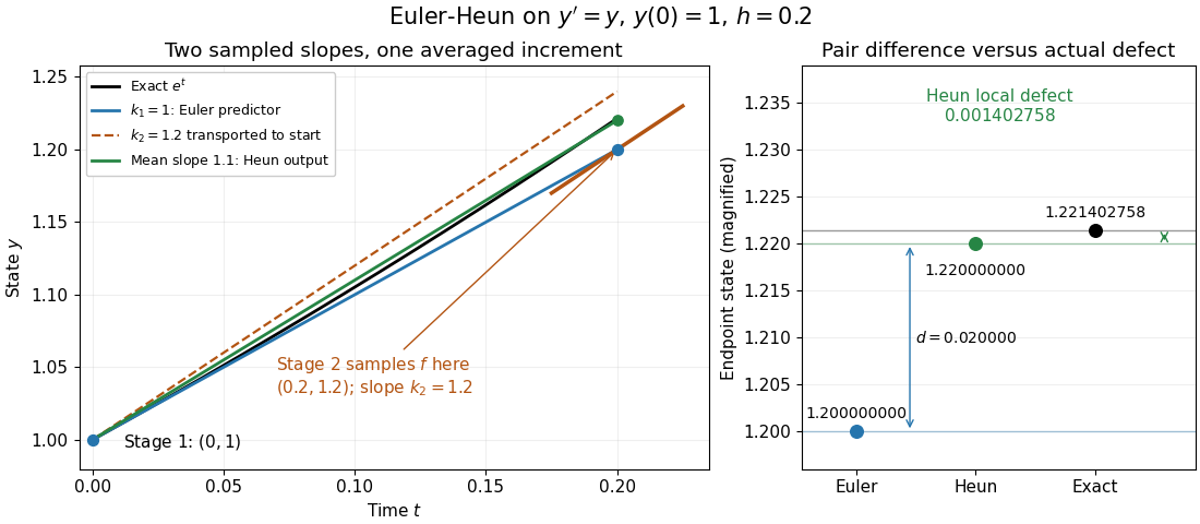
Euler-Heun stage geometry for y prime equals y: sample at the Euler predictor, then average slopes for the corrected endpoint
. Details. 
For , and , the sampled slopes are and . Transporting the second slope to the starting point would end at ; the average slope instead ends at . The exact exponential function reaches . The magnified endpoint comparison separates the pair difference from the actual Heun local defect .
An -stage Runge-Kutta method has stability function , a rational function with numerator and denominator degrees at most . Order forces , so uniqueness of the diagonal Padé approximant identifies with . That approximant has no poles in the closed left half-plane and modulus at most one there. Hence every such maximal-order method is A-stable. Since the Padé approximant numerator and denominator are coprime and both have degree , the original stage determinant cannot have hidden canceled poles in that half-plane.
This one-step family interpolates between the Forward Euler method at , the trapezoidal rule at , and the Backward Euler method at . Its stability function is . It is first order except at one half, where it is second order. Applying it to spatial diffusion gives the theta diffusion stability criterion.
On an orthogonal diffusion eigenmode, the theta method has the displayed amplification with . The identity proves contraction at all nonnegative exactly when . For , contraction holds up to , with a positive denominator in that range. Orthogonality is what transfers these modal bounds to a full L2 norm estimate.
At , arbitrarily stiff heat modes approach amplification : the Crank-Nicolson method is contractive but does not rapidly damp unresolved rough components. The Backward Euler method instead has limit zero. Thus unconditional linear stability and strong stiff decay are different requirements. High smooth-data consistency order alone does not imply a uniform high-order estimate down to the initial instant for arbitrary L2 initial conditions.
A strong stability preserving Runge-Kutta method writes its stages as convex combinations of previously computed states and suitable Forward Euler method steps. It transfers any convex-functional nonincrease property of the forward step, such as a norm bound, under a proportionally scaled time-step restriction.
For example, if is nonexpansive in a norm, then and is also nonexpansive: the triangle inequality bounds the new difference by one half of the initial difference plus one half of the twice-advanced difference. Both are at most the initial difference. A Taylor expansion yields , so this is a second-order Runge-Kutta method. The forward-step hypothesis must hold on the stage states; preservation of one chosen convex bound is not the same as unconditional B-stability.
The classical four-stage explicit Runge-Kutta method usesIt satisfies the fourth-order conditions for a Runge-Kutta method. Its polynomial stability function excludes A-stability, while gives the imaginary-axis stability interval .
A Butcher tableau records a Runge-Kutta method's stage matrix , time nodes , and output weights in the block arrayRead row above the line as the recipe for Runge-Kutta stage : the left entry gives , and the right entries give the coefficients in . Below the line, weights slope in the final update. Zeros on and above the diagonal identify an Explicit Runge-Kutta method. For the internally consistent convention, row sums of equal ; first-order consistency of a numerical method also requires . An embedded Runge-Kutta pair adds another weight row while retaining .
A Butcher order condition equates the coefficient assigned by a Runge-Kutta method to a rooted tree with the corresponding exact Taylor coefficient. Satisfying every condition through tree order is equivalent to Runge–Kutta order at least .
For a general nonautonomous Runge-Kutta method, Taylor expansion of stage gives . Matching the exact increment gives the three displayed conditions. When internal consistency is imposed, the last two coincide. Internal consistency is a usual tableau convention, but is not logically necessary for order two of a generalized tableau.
With and , a Runge-Kutta method has order at least four exactly when the eight Butcher order conditionshold; powers of are componentwise. These conditions match the numerical and exact coefficients indexed by rooted trees through order four. Matching the scalar Dahlquist test equation alone is insufficient to check the nonlinear Butcher order conditions.
An implicit Runge-Kutta method defines one or more stages through equations involving those same stages.
For stages and with update , the method has order two for every fixed real . The third-order coefficient of is always , not , so no parameter gives third order on general nonlinear equations. The displayed stability function is bounded throughout the left half-plane only when , when it is the A-stable trapezoidal function . It is not L-stable.
For a vector field uniformly Lipschitz continuous in the state with constant , the stage fixed-point map of an implicit Runge-Kutta method is a contraction in the maximum stage norm if . The contraction mapping theorem then gives unique stages. This is a sufficient small-step condition; a dissipative vector field may permit solvability for larger steps. An algebraic stability or B-stability estimate compares existing stage solutions and should not be mistaken for an unqualified stage-existence theorem.
The implicit midpoint rule advances an autonomous ordinary differential equation byIt is a second-order, A-stable, time-symmetric numerical method.
The implicit midpoint rule is the midpoint method with . It is a one-stage implicit Runge-Kutta method.
For a uniformly Lipschitz continuous state field with constant , an implicit midpoint rule step is uniquely solvable when , by the contraction mapping theorem. Write its step map as , where . Subtracting the increment equations givesTherefore , and the triangle inequality gives the bound for . Combining it with the implicit midpoint consistency bound yieldsfor . This follows by summing the geometric error recurrence with forcing . For and , , proving second-order global error with exact starting data. If , the direct bound is .
For an exact solution , define the normalized local truncation error of the implicit midpoint rule byIf , and the state Jacobian matrix of has operator norm at most on the intervening state segments, then the displayed bound holds uniformly on a fixed finite interval. To prove it, put . Symmetric Taylor expansions giveFor the first bound, integrate the second-order remainder of over the symmetric step; for the second, average the second-order remainders of at the endpoints. The odd terms cancel. The Lipschitz condition for and finish the proof by the triangle inequality. The unnormalized step residual is .
The Crank--Nicolson method applies the trapezoidal rule to a semidiscrete evolution equation. For a linear system its update is
For symmetric negative semidefinite matrices , each factor has norm at most one, since its eigenvalues are with . The same holds for , so their ordered product is a contraction for every , whether or not commute. This proves unconditional discrete L2 norm stability of the split Crank-Nicolson method for directional diffusion. Its splitting error remains first order in general, because the product's quadratic defect is .
Given distinct nodes , a collocation Runge-Kutta method uses the Lagrange basis with and . Its stages enforce the differential equation at the collocation nodes.
This applies the collocation method to the time-step polynomial of an ordinary differential equation.
For distinct nodes , the two-stage collocation Runge-Kutta method has stability functionThe denominator has no zeros in the closed left half-plane. On the imaginary axis the denominator's squared modulus minus the numerator's is . Thus , equivalently , is necessary and sufficient for A-stability, using the maximum modulus principle and the bound at infinity.
For distinct collocation nodes, let . If for , and the next moment is nonzero, the associated interpolatory quadrature has order , and the collocation Runge-Kutta method has the same classical order for sufficiently smooth differential equations. Here . Equivalently, if the quadrature is exact through degree but not degree , the method has order . The generic order is at least , Gauss collocation methods reach , and Radau IIA methods reach .
For collocation nodes, the residual of the collocation polynomial vanishes at each node and contains the factor . Quadrature exactness through degree implies for every polynomial of degree at most . Expand the smooth vector-field interpolation error and the derivative of the exact flow in powers of the step. Every endpoint-error term of degree below has this vanishing weighted moment, so the endpoint local error is , although the interior stage accuracy is generally only . A step Lipschitz estimate and discrete Gronwall inequality then give global order . Gaussian nodes attain , while the first nonexact quadrature moment bounds the order from above.
For a collocation Runge-Kutta method, , where the Lagrange interpolation basis obeys . Hence each row sum is its collocation node. Failure of this identity disproves a claimed collocation tableau with those nodes. The identity alone is necessary rather than sufficient: the individual integrated basis coefficients must also agree.
A Lobatto IIIA method collocates at the Lobatto quadrature nodes, including both endpoints of the time interval. Its three-stage version hasThe Butcher order conditions give order four. Its stability function iswhich is A-stable but not L-stable. It is not algebraically stable: the first diagonal entry of the defining matrix is . This distinguishes linear A-stability from nonlinear algebraic stability.
The -stage Gauss--Legendre Runge--Kutta method collocates at the Gauss--Legendre quadrature nodes on . It is symmetric, A-stable, and has order .
Choose as the polynomial roots of in , and form the Lagrange interpolation polynomials . The Gauss collocation method has and . This gives explicit coefficient formulas after finding polynomial roots: if , these integrals are and . Gaussian quadrature gives order .
The two-stage Gauss--Legendre Runge-Kutta method uses nodes , weights and coefficients , , . The Butcher order conditions give order four. Its stability function is the displayed rational function, which is A-stable. The algebraic stability matrix is zero, so positive weights also give nonlinear contractivity for dissipative vector fields.
An -stage Radau IIA method collocates at the right-endpoint Radau nodes. It has order and is both algebraically stable and L-stable.
Suppose an -stage Runge-Kutta method has order , an invertible matrix , and . Its stability function is . The adjugate matrix formula gives a rational function with denominator degree and numerator degree at most ; its zero limit at infinity lowers the latter degree to at most . The order of a numerical method gives , identifying the Padé approximant. Uniqueness follows because the cross-multiplied difference of two candidates has degree at most but a zero of order at least , so is identically zero. The A-stability of near-diagonal exponential Padé approximants then proves A-stability, and the zero limit proves L-stability. These conditions identify the stability function; they do not alone claim uniqueness of all entries of the Runge-Kutta method tableau.
A Runge-Kutta method is algebraically stable when and the matrix with is positive semidefinite. Algebraic stability implies contractivity for dissipative differential equations.
For stage states and a vector field with , expansion of the new squared norm gives , where . Hence preserves the quadratic form exactly for every well-defined step. The same argument with a fixed symmetric matrix in the inner product preserves any quadratic invariant of the vector field. In particular it preserves the Euclidean norm for a skew-symmetric matrix differential equation.
An algebraically stable Runge-Kutta method is B-stable: for a dissipative vector field, a well-defined step cannot increase the distance between two starting values. This assumes that the compared stage equations have solutions, as required by stage solvability of an implicit Runge-Kutta method. The Runge-Kutta contractivity identity expresses the distance change as a nonpositive weighted term coming from the dissipative vector field minus a nonnegative quadratic form involving the matrix defining algebraic stability. Positive weights also rule out stage poles in the open left half-plane on the scalar test equation, giving A-stability there; zero-weight redundant stages need separate solvability attention.
For differences between corresponding stages and differences between their vector fields, a Runge--Kutta step satisfiesTo derive the identity, expand the squared norm of and substitute in the linear term. Symmetrizing the double sum gives the displayed coefficients . For a dissipative vector field, the first sum is nonpositive when , and the second sum is nonnegative when the matrix is a positive semidefinite matrix. Thus algebraic stability implies B-stability.
As a quadrature rule, the trapezoidal rule replaces an integrand by the linear interpolation joining its two endpoint values:For nonnegative endpoint values, this is the area of a trapezoid; in general it is a signed area. The quadrature nodes are , each with quadrature weight . Unlike the midpoint quadrature rule, it uses endpoint samples, which can be reused between adjacent panels.
Every affine function agrees with its linear interpolation, so the trapezoidal rule integrates it exactly. On , gives . On , the polynomial instead gives , exceeding by . Its degree of precision of a quadrature rule is exactly one.
If , its signed approximation error satisfiesA convex function lies below its endpoint chord, so the trapezoidal rule overestimates its integral; a concave function gives the reverse inequality. The error formula assumes that the second derivative exists and is a continuous function throughout the closed interval.[ref]
3.5 Quadrature, subsection (i) Trapezoidal Rules. §3.5(i), equation 3.5.1 and its C² hypothesis; the source writes integral minus rule
A short derivation is the identityobtained by two integrations by parts. The nonnegative Peano kernel has integral , and the weighted mean value theorem for integrals gives the formula.The trapezoidal rule for an ordinary differential equation averages vector fields at the old and new states and is A-stable.
This time-stepping use applies the same trapezoidal rule to the integral of the derivative in an ordinary differential equation. That connection explains its place under implicit Runge-Kutta methods; its quadrature behavior and the nonlinear issue in trapezoidal rule fails B-stability concern different uses of the same endpoint averaging.
For with , the trapezoidal rule satisfies the displayed bound, and the constant is best possible. The polynomial interpolation error for the endpoint linear interpolant satisfies , where . Integrating this inequality and using the triangle inequality for an integral proves the bound because . Equality holds for : the exact integral is , its trapezoidal rule estimate is , and .
On an equal-panel partition of an interval, with , sum the trapezoidal rule over adjacent panels:There are distinct quadrature nodes. Each interior sample belongs to two panels and therefore has quadrature weight , while each endpoint has quadrature weight . Equivalently, the composite trapezoidal rule integrates the piecewise linear function obtained by linear interpolation exactly.[ref]
For and , summing panel quadrature errors givesfor some . Thus panel quadrature errors of order accumulate to order , using big O notation.[ref]
3.5 Quadrature, subsection (i) Trapezoidal Rules. §3.5(i), equations 3.5.2–3.5.3: composite formula and signed error
On a nonuniform partition of an interval with widths and largest width , the bound is .For the polynomial on , direct summation yieldsBoth quadrature errors shrink by exactly four when doubles, with opposite signs. This exact relation belongs to this polynomial example; the trapezoidal rule is not always twice as inaccurate as the midpoint quadrature rule.
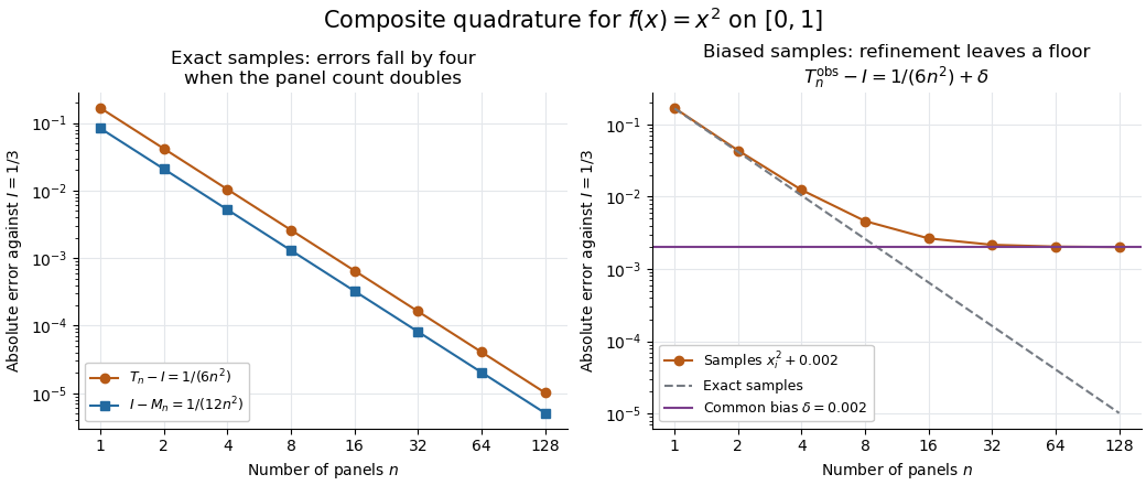
Quadratic quadrature errors fall by four on refinement while a common sample bias persists
. Details. 
The left plot uses exact polynomial sums; the right adds a common sample bias to the composite trapezoidal rule. That mathematical model converges to , showing why smaller panels alone do not ensure accuracy for noisy samples. It illustrates noise sensitivity of a quadrature rule, rather than measured data.
On a partition of an interval symmetric about zero, the composite trapezoidal rule gives opposite quadrature nodes equal quadrature weights. Samples of an odd function cancel pairwise, and a zero quadrature node contributes zero. For a continuous odd function, its exact integral over is also zero. Adding any affine function preserves exactness by linearity of the integral and of the quadrature rule. For example, is nonpolynomial but both the exact integral and every uniform-grid composite trapezoidal rule value on are two.
On a uniform partition of with width , the right Riemann sum and the composite trapezoidal rule have equal weights at every interior mesh point. They differ only by adding half a final-endpoint weight and removing half an initial-endpoint weight. This proves the displayed identity. For continuous , both converge to its definite integral; their finite endpoint correction need not be confused with the smaller trapezoidal discretization error for a smooth integrand.
If is twice continuously differentiable on , take a uniform bound . On one panel , two integrations by parts give the signed quadrature errorThe nonnegative kernel has integral , so the absolute error is at most . Summing equal panels proves the displayed bound. The maximum exists on the closed interval; a supremum or any known uniform bound also suffices. The estimate certifies a sufficient panel count, which need not be the least count achieving a particular actual error.
The trapezoidal rule is A-stable but is not B-stable. For the dissipative vector field at step size one, its uniquely defined step map obeys . At , and implicit differentiation gives , so nearby states expand rather than contract. This is a concrete nonlinear obstruction, rather than merely failure of the sufficient algebraic stability criterion.
A one-step numerical method with step map is time symmetric when . Its leading local-error power is odd, so every nontrivial consistent time-symmetric method has even order.
The order is the highest power through which the one-step expansion matches the exact Taylor expansion.
For an explicit Runge-Kutta method with coefficients , put and let mean componentwise squaring. The conditions , , and match the exact flow expansion through degree three: the two cubic differentials are and . For sufficiently smooth vector fields these give local error and, under the usual finite-interval Lipschitz continuity assumptions, global error .
Articles by others on the same topic
There are currently no matching articles.