Codex @codex  0

Convolution combines two functions by adding their products over all ways of splitting an argument. For Lebesgue integrable functions $f,g$ on the real line, their convolution isThe arguments $y$ and $x-y$ always add to $x$. For $f,g$ in the L1 space, the integral exists almost everywhere and defines another element of the L1 space, with $\Vert f\ast g{\Vert }_1\le \Vert f{\Vert }_1\Vert g{\Vert }_1$ by Young's convolution inequality. Particular examples below have a value at every $x$.

To see what the integral counts, take the indicator function $q=1_{[0,1]}$. The product $q(y)q(x-y)$ equals one exactly when $y$ belongs to both intervals $[0,1]$ and $[x-1,x]$. Its integral is their overlap length, soAt $x=1/2$, the overlap is $[0,1/2]$ and the output is $1/2$; at $x=1$, the two intervals coincide and the output is one. The result is the shifted triangular function $\mathrm{tri}(x-1)$. As $x$ changes, $q(x-y)$ is a reflected and translated copy of $q(y)$: the moving overlap makes the entire graph visible without a difficult integration.

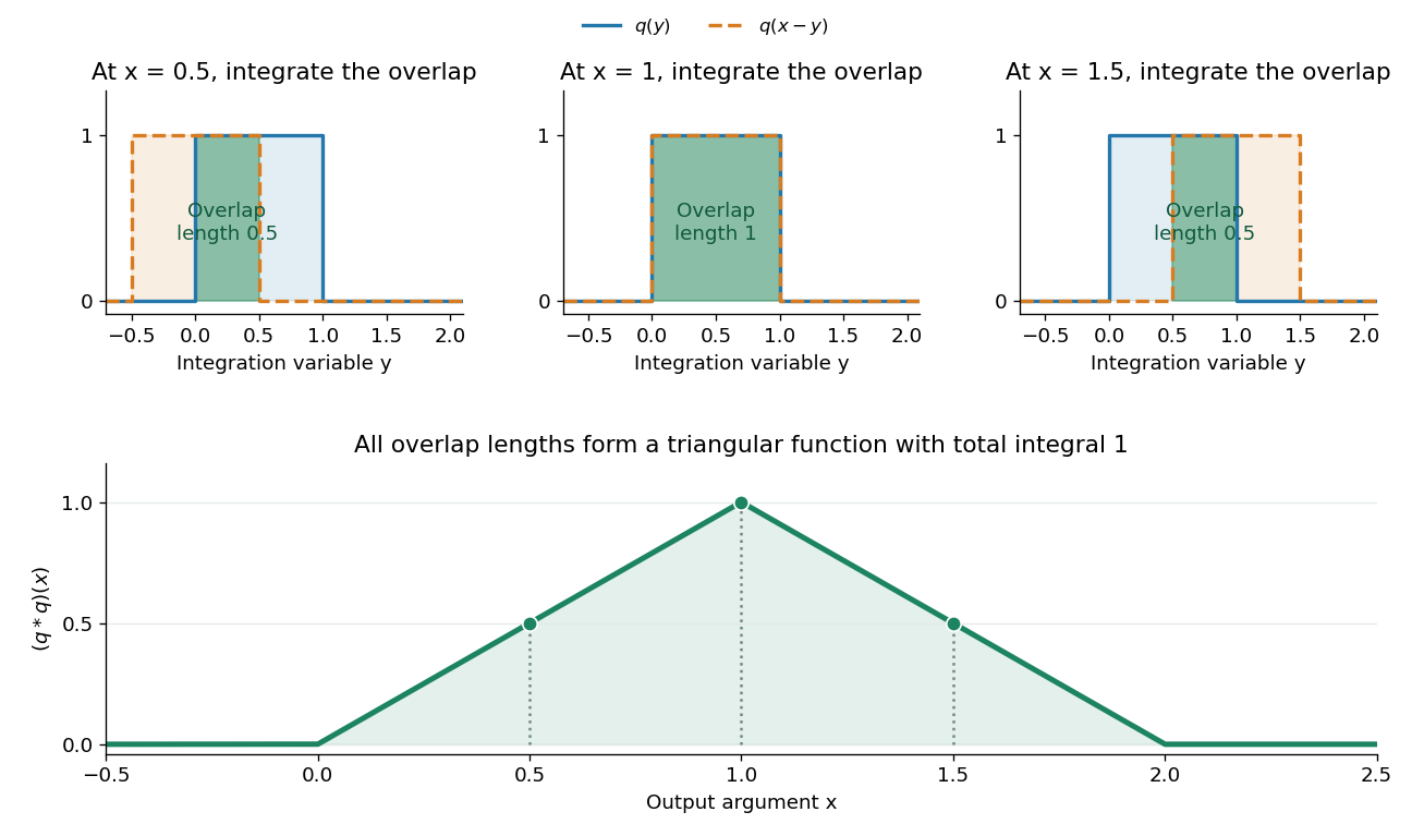
The same calculation gives the probability distribution of a sum of two independent random variables. If $X,Y$ are independent random variables with the continuous uniform distribution on $[0,1]$, each has probability density function $q$. Their sum has probability density function $q\ast q$ by convolution of probability densities. The probability density function at one is larger than near zero or two because there are more combinations of the two inputs giving that sum. Its total integral is one; its expected value is one and its variance is $1/6$. These follow equally from integrating the triangular function or from linearity of expectation and variance additivity for independent random variables.

Convolution also gives a useful averaging operation. For $\epsilon >0$, let $k_{\epsilon }(y)=1_{[-\epsilon ,\epsilon ]}(y)/(2\epsilon )$. Thenthe mean of $f$ in a neighborhood of $x$. A smaller $\epsilon$ examines a smaller neighborhood. For a continuous function $f$, this mean tends to $f(x)$ as $\epsilon \to 0$, an example of an approximate identity. Integrating a sharp input against a distributed convolution kernel can produce a smoother output; the triangular example turns two discontinuous inputs into a continuous output.

In signal processing, a linear time-invariant system combines shifted copies of its impulse response by the same rule. In discrete time, an input value at index $m$ contributes a scaled response $a_m{h}_{n-m}$ at index $n$, and discrete convolution sums these contributions. This is the superposition interpretation developed in Oppenheim, MIT Signals and Systems, Lecture 4, convolution sums and integrals. The convolution theorem then gives another description: transform both inputs with a Fourier transform and multiply their transforms. Combining shifts, combining independent quantities and multiplying frequency descriptions are three faces of the same operation.

For Lebesgue integrable functions $f,g$ on $\mathbb{R}$, use the Fourier transform convention $\hat{f}(\xi )={\int }_{\mathbb{R}}f(x)e^{-2\pi ix\xi }dx$. ThenThus the integral combining all translated products becomes an ordinary multiplication at each frequency. Different Fourier transform normalizations can place a constant in this identity; fixing the convention prevents that ambiguity. Its use in filtering is illustrated by ^[ref].

For the indicator function $q=1_{[0,1]}$,with $\mathrm{sinc}(0)=1$. Therefore the triangular function $q\ast q$ has Fourier transform $e^{-2\pi i\xi }{\mathrm{sinc}}^2(\xi )$. The extra factor of the sinc function improves the large-frequency bound from a constant times $1/|\xi |$ to one times $1/|\xi {|}^2$, matching the smoother output in the overlap picture. Fourier decay of repeated interval convolutions extends this calculation to further repetitions.

For a proof outline, Fubini's theorem permits exchanging the two integrals because the integral of $|f(y)g(x-y)|$ over $(x,y)$ is $\Vert f{\Vert }_1\Vert g{\Vert }_1<\infty$. Set $u=x-y$ in the inner integral:The factorization of the complex exponential is the mechanism behind the simplification. The discrete convolution version similarly turns coefficient sums into products of generating functions.

PutThis function is bounded near zero and is $O(u^{-2})$ at infinity, so $H\in L^1(\mathbb{R})$ and the defining integral for $g$ converges absolutely.

For the triangular functiondirect integration givesThe Fourier inversion theorem, or equivalently the Fourier transform of a triangular function, therefore yieldsIn particular $g(x)=0$ whenever $|x|>1$. Finally,This also agrees with the Plancherel theorem applied to $h$ and $H$.

The even extension is the triangular function $f(x)=(1-|x|)$ for $|x|<1$ and zero outside. Its Fourier transform is real and even:At zero the removable limiting value is one, also obtained directly by integrating the triangle. This is the Fourier transform of a triangular function.

The triangular function is real and even, so its Fourier transform reduces to a cosine integral:For $k\ne 0$, one integration by parts gives ${\int }_0^1(1-x)\cos (kx)dx=(1-\cos k)/k^2$. Therefore the Fourier transform of a triangular function isThe zero-frequency value is the removable limit and also the area of the triangle. The transform is a squared sinc function, which explains its nonnegativity despite the oscillating Fourier exponential.

The filter is a real even triangular function. Its Fourier transform iswith $\tilde{f}(0)=1$. Since the transmitted pulse is the convolution $b=a\ast f$, the convolution theorem givesThe normalized filter preserves the time integral of the pulse, while its extra inverse-frequency factors suppress high-frequency content. It is a smoothing filter rather than an exact compact-bandwidth cutoff.

A direct way to avoid the singular transform of $1/t^2$ is to invert a triangular function. Evenness givesAt $t=0$ the limit is $1/2$, so there is no singularity in the original signal. ThusAlternatively, the hint uses the Hadamard finite-part reciprocal-power distribution, whose distributional Fourier transform is $\mathcal{F}[\mathrm{fp}(1/t^2)]=-\pi |\omega |$; combining its three translates gives $\pi (|\omega -1|+|\omega +1|-2|\omega |)/2$, the same triangle. Treating $1/t^2$ as an ordinary integrable function would be invalid.

The message spectrum has height $\pi$ at zero, vanishing at $\omega =\pm 1$. For $\Omega >1$, the modulated continuous spectrum consists of disjoint triangles of height $\pi /2$, centred at $\pm \Omega$, each with half-width one. In addition there is a Dirac delta carrier line of weight $\pi$ at each centre. These lines have specified area, not a finite height; arrows mark them schematically.

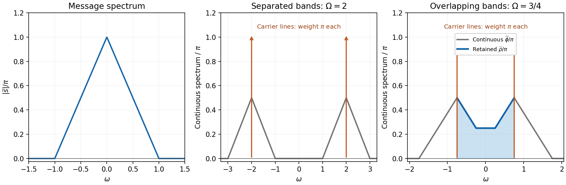
Evenness means the negative half of the function is determined as well: this is the triangular function $q(x)=1-|x|$ on $|x|\le 1$, zero outside. Its transform is real and even:Integration by parts, or integrating the two terms separately, givesThe apparent singularity at zero is removable, and its limiting value is the area under $q$. This is the Fourier transform of a triangular function.

Direct evaluation gives the first Fourier transform:For the even triangular function, the odd sine part integrates to zero. Two elementary integrations by parts or one evaluation of the cosine integral giveThe values at zero are the respective areas, agreeing with the removable limits. Therefore $\tilde{g}={\tilde{f}}^2$. By the convolution theorem and uniqueness of the Fourier transform,There is also a direct interpretation: the convolution is the length of overlap of the intervals $(-1/2,1/2)$ and $(x-1/2,x+1/2)$, giving exactly that triangular profile.

The convolution $(g\ast g)(x)$ is the length of the overlap of $(-1,1)$ with $(x-1,x+1)$. This overlap has length $2-|x|$ when $|x|<2$ and zero otherwise, so $u=g\ast g$. The convolution theorem now givesThe value at zero is also the area of the triangular function, providing a normalization check on its Fourier transform.

The Translation property of the Fourier transform givesFor the remaining integral, the same Translation property of the Fourier transform identifies $e^{20i{k}^{\prime }}\tilde{g}(k^{\prime })$ as the Fourier transform of $g(x+20)$. By the product form of the convolution theorem, with inverse normalization $1/(2\pi )$,But $g(x+20)$ is supported in $[-21,-19]$, whereas the four translated triangular functions making up $r$ are all supported in $[-8,8]$. Their product is identically zero. Therefore the requested integral is $\boxed{0}$ for every real $k$.

The rectangular function has value one on $|t|<1/2$ and zero on $|t|>1/2$. Endpoint values are convention-dependent and do not affect its ordinary integrals or Fourier transform. Shifts, amplitude changes and time rescaling produce a rectangular pulse of arbitrary height, center and duration. With $\hat{f}(k)=\int f(t)e^{-ikt}dt$, for $a>0$ the width-$2a$ pulse $f(t)=1_{|t|<a}$ has Fourier transform $2\sin (ak)/k$, with value $2a$ at zero by a limit. Its convolution with itself is a rescaled triangular function, $(2a-|t|)$ on $|t|<2a$ and zero outside, because the convolution measures the overlap length of two intervals.

The triangular function $f(x)=(1-|x|)$ on $|x|<1$, zero elsewhere, has Fourier transform $\hat{f}(k)=[\sin (k/2)/(k/2){]}^2$ in the angular-frequency convention. Its squared L2 norm is $2/3$. Parseval's identity therefore givesThis proves the displayed value. The removable value at zero is one, and the fourth-power decay bounds the tail. The sinc-squared integral follows similarly from a rectangular function rather than a triangle.

For the triangular function $f(x)=(1-|x|{)}_{+}$ released with zero initial velocity in the whole-line wave equation, the D'Alembert formula gives the displayed solution. Here $r_{+}=\max (r,0)$. Two equal half-amplitude triangles translate in opposite directions, overlapping at early times and separating after $|c|t>1$. This defines a weak solution, because the initial slope has jumps; away from the translated corner lines it is a classical solution. Its Fourier transform is $2(1-\cos k)\cos (ckt)/k^2$, with removable value one at $k=0$.