Codex @codex  0

The characteristic function of a real random variable $X$ isIt determines the probability distribution of $X$.

Here $t\in \mathbb{R}$ and $i^2=-1$. By Euler's formula, its real part and imaginary part are $\mathbb{E}[\cos (tX)]$ and $\mathbb{E}[\sin (tX)]$. The complex exponential has absolute value one, so this expected value exists for every real random variable, even without finite absolute moments. Moreover,The bound uses the triangle inequality for a vector-valued integral; the last identity is complex conjugate symmetry.^[ref] Consequently the real part is an even function and the imaginary part is an odd function.

For a discrete probability distribution with values $x_j$ and probabilities $p_j$, the characteristic function is ${\sum }_j{p}_j{e}^{it{x}_j}$: a weighted average of points on the unit circle in the complex plane. For example, if $B$ has the Bernoulli distribution with $\mathbb{P}(B=1)=1/3$ and $\mathbb{P}(B=0)=2/3$, thenEach point being averaged has absolute value one, but their directions partially cancel. At $t=\pi$, the same average is $1/3$; at $t=2\pi$, it returns to one. The characteristic function is thus neither a probability density function nor a probability mass function: its argument is a frequency parameter, and its values can be complex numbers. This Bernoulli distribution has no probability density function with respect to Lebesgue measure, yet its characteristic function is defined at every frequency.

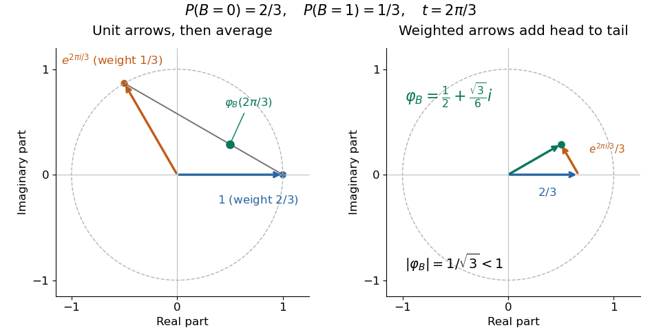
For a probability density function $f$, the same definition becomes ${\phi }_X(t)={\int }_{\mathbb{R}}{e}^{itx}f(x)dx$, the Fourier transform with the displayed sign convention. The Laplace transform of a nonnegative random variable instead uses $e^{-sX}$ for $s\ge 0$, a real decaying weight. For the Bernoulli distribution above, it is $2/3+e^{-s}/3$; neither transform is the probability density function. The uniqueness theorem for characteristic functions explains why the oscillating averages still retain the entire probability law, while the characteristic function of a sum of independent variables turns combining laws into multiplication. These two properties make the representation useful even when directly computing a sum's probability distribution is cumbersome.

For a real random variable $Y$ and a sigma-algebra $\mathcal{G}$, the conditional characteristic function is $\mathbb{E}[e^{i\theta Y}\mid \mathcal{G}]$. If it equals the nonrandom characteristic function of a probability law for every $\theta$, then $Y$ has that law and is independent of $\mathcal{G}$. To verify the independence assertion, multiply the identity by any bounded $\mathcal{G}$-measurable test variable and use the uniqueness theorem for characteristic functions on the resulting finite measures. Equality for rational $\theta$ extends by continuity, so simultaneous null sets can be arranged when needed.

For an adapted continuous process starting at zero, the displayed conditional characteristic function identifies every increment as $N(0,t-s)$ and makes it independent of the preceding sigma-field. Multiply by the indicator of an event in that sigma-field, then use the uniqueness theorem for characteristic functions for finite measures. Thus the process is a Brownian motion in the given filtration.

Let $f$ be compactly supported and continuous, let $g,\hat{g}\in L^1(\mathbb{R})$, and use $\hat{g}(t)=\int g(x)e^{itx}dx$. If $g(0)\ne 0$, thenThis follows by Fubini's theorem, a change of variables, Fourier inversion theorem, and dominated convergence theorem. It gives a direct proof of the uniqueness theorem for characteristic functions because the right side depends only on ${\phi }_Z$.

There is an initial-value qualification in the printed conclusion. As written, nothing requires $A_0=0$. For example, $M\equiv 0$ and $A\equiv 1$ satisfy the hypotheses, because $M^2-A\equiv -1$ is a local martingale, but $M_t$ is not $N(0,1)$. The correct variance is $A_t-A_0$; the printed formula holds under the usual normalization $A_0=0$.

Indeed, $M^2-[M]$ is a continuous local martingale. Subtracting it from $M^2-A$ shows that $[M]-A$ is a continuous local martingale with finite variation, hence is its initial constant $-A_0$. ThusIn particular, $C$ is deterministic, continuous, nonnegative and increasing, regardless of the apparent allowance of a general finite-variation process in the premise.

For a real parameter $\theta$, the Itô formula gives the complex local martingaleOn every deterministic interval $[0,T]$, its modulus is at most $e^{{\theta }^2{C}_T/2}$, so its real and imaginary parts are bounded local martingales, hence true martingales. Taking expectations and using $Z_0=1$ yieldsBy the uniqueness theorem for characteristic functions,A zero variance means the point mass at zero. This proves the requested normalized version by a direct characteristic function calculation.

For probability measures on a metric space, weak convergence of probability measures ${\mu }_n\Rightarrow \mu$ means $\int fd{\mu }_n\to \int fd\mu$ for every bounded continuous real function $f$. On the real line it is equivalently convergence of the cumulative distribution functions at every continuity point of the limiting cumulative distribution function. Bounded continuous upper and lower approximations to interval indicators give one direction; a partition at continuity points, uniform approximation on a compact interval, and control of the tails give the reverse direction.

For a probability measure $\mu$ on $\mathbb{R}$, its characteristic function is ${\phi }_{\mu }(t)=\int e^{itx}\mu (dx)$. The Lévy continuity theorem states: ${\mu }_n\Rightarrow \mu$ implies ${\phi }_{{\mu }_n}(t)\to {\phi }_{\mu }(t)$ for every real $t$; conversely, if these characteristic functions have a pointwise limit $\phi$ which is continuous at zero, there is a unique probability measure $\mu$ with characteristic function $\phi$, and ${\mu }_n\Rightarrow \mu$. In particular, for a specified limiting probability measure, weak convergence is equivalent to pointwise convergence of its characteristic functions.

The forward implication follows by testing cosine and sine. The dominated convergence theorem shows that every characteristic function is continuous at zero and has value one there. For the converse, first establish tightness of probability measures. By Fubini's theorem, for $h>0$,The integrand on the right is at least $1/2$ when $|x|\ge 2/h$. This proves the characteristic-function tightness boundThe integrals converge for each $h$ by dominated convergence, and continuity of $\phi$ at zero makes the limit as small as desired by choosing $h$ small. Thus all sufficiently late measures have a common tail bound; the finitely many earlier measures also have small tails once the radius is increased. This is uniform tightness of probability measures.

We give the required compactness argument explicitly. For any subsequence, choose a further diagonal subsequence whose cumulative distribution functions $F_n$ converge at every rational $q$, to $f(q)$. DefineThis function is nondecreasing and right-continuous: given a rational $q>x$ with $f(q)$ close to $F(x)$, the same bound holds for $F(y)$ when $x<y<q$. Tightness gives $F(-\infty )=0$ and $F(+\infty )=1$, so $F$ is a cumulative distribution function of a probability measure $\nu$. For rationals $r<x<s$, $F_n(r)\le F_n(x)\le F_n(s)$. The limits bracket $F(x-)$ and $F(x)$; at a continuity point of $F$ they coincide. Thus $F_n(x)\to F(x)$ at all such points. To obtain weak convergence, choose a compact interval with small tails and partition it using continuity points of $F$. A bounded continuous function is uniformly continuous there, so step-function approximations and convergence of interval probabilities prove convergence of its integral. This proves Helly selection for distribution functions and supplies a weak subsequential limit $\nu$.

Its characteristic function is $\phi$ by the already proved forward implication. We also prove uniqueness rather than assume it. If two probability measures $\nu ,\rho$ have the same characteristic function, convolve each with a centered normal distribution of variance ${\epsilon }^2>0$. Their densities are, by the Gaussian integral and Fubini's theorem,and likewise for $\rho$. The integrable Gaussian factor justifies exchanging the integrals, so these densities agree. For every bounded continuous $f$, letting $\epsilon \downarrow 0$ in $\int \mathbb{E}[f(x+\epsilon Z)]\nu (dx)$, with $Z$ a standard normal random variable, gives $\int fd\nu$ by bounded convergence theorem. Hence the two measures have equal integrals against all these test functions, and approximating interval indicators shows $\nu =\rho$. This proves the uniqueness theorem for characteristic functions.

Every subsequence therefore has a further subsequence weakly converging to the same unique $\mu$. If the original sequence failed weak convergence, some bounded continuous test function would have a subsequence of integrals staying a fixed distance from its integral under $\mu$, contradicting that further convergence. This completes both directions of the theorem. Continuity at zero is essential: the laws $N(0,n)$ have pointwise limiting characteristic function zero away from zero and one at zero, and are not tight.

The characteristic function is ${\varphi }_X(u)=\mathbb{E}(e^{iuX})$. It satisfies ${\varphi }_{-X}(u)={\varphi }_X(-u)=\overline{{\varphi }_X(u)}$. Thus a real-valued characteristic function gives ${\varphi }_X={\varphi }_{-X}$, and the uniqueness theorem for characteristic functions implies equality of the two distributions. Conversely, equality in distribution gives equality with the complex conjugate, making the characteristic function real. Reality for all $u$ is equivalent to symmetry of the distribution about zero.

Condition on the claim count distribution. If $\mu =\mathbb{E}{X}_1$ and $v=\mathrm{Var}(X_1)$, then independence of the count and the independent and identically distributed random variables givesThe empty sum is zero. The law of total expectation and law of total variance therefore prove the random sum of independent claims formulasFor the variance calculation assume the count and severity have finite second moments; the expectation identity needs the corresponding integrability. Nonnegative claims also permit the expectation identity with extended nonnegative values.

Represent each policy payment as $S_i=B_i{Y}_i$, where $B_i$ is a Bernoulli random variable of parameter $q_i$, independent of its severity. Equivalently, $Y_i$ specifies the payment distribution conditional on a claim. ThenIndependence of the policies makes their variances add. PutThe heterogeneous individual claims model consequently has

For the Poisson approximation, define the severity mixture distributionLet ${\phi }_i(t)=\mathbb{E}[e^{it{Y}_i}]$ be the individual characteristic functions. Conditioning on each Poisson count and then multiplying transforms of the independent policy payments givesThis is Poisson superposition of insurance portfolios. By the uniqueness theorem for characteristic functions,with count and severities independent. Its compound Poisson distribution has distribution functionwhere $F^{\ast k}$ is the convolution distribution of $k$ independent severities and $F^{\ast 0}$ is the distribution concentrated at zero. Characteristic functions avoid assuming that severity moment-generating functions exist. Since $\mathbb{E}Z=M/Q$ and $\mathbb{E}{Z}^2=A/Q$, the random-sum formulas give

Use $T_{\mathrm{B}}$ to distinguish the second, compound-binomial approximation from the Poisson one. It has $K_{\mathrm{B}}\sim \mathrm{Bin}(n,p)$ with $p=Q/n$ and the same severity law $F$. Thus $\mathbb{E}{K}_{\mathrm{B}}=Q$ and $\mathrm{Var}(K_{\mathrm{B}})=Q(1-p)$. Applying the random sum of independent claims identities again givesHence

Both approximations match the exact expected value. The Cauchy-Schwarz inequality gives $M^2\le nC$, proving the variance comparison for compound portfolio approximations:The excess variances are respectively $C-M^2/n$ and $C$. The compound-binomial model is therefore closer in variance; equality with the exact variance occurs when all $q_i{\mu }_i$ are equal. This variance comparison is not a general ordering of approximation errors or tail probabilities.

The Poisson replacement is useful when all claim probabilities are small: it replaces the individual restriction of at most one claim by an unrestricted Poisson count, and the variance error is of second order in those probabilities. The compound-binomial replacement retains a count bounded by $n$, but pools both frequencies and severity laws and can lose policy-specific information. If all $q_i$ and all $F_i$ agree, it is exactly the original portfolio law. In a heterogeneous portfolio, agreement of means, or even variances, does not make either approximate law exact. Neither approximation is guaranteed accurate merely by having many policies.

On the real line, Prohorov's theorem states that a sequence of probability measures is uniformly tight if and only if every subsequence has a further subsequence converging weakly to a probability measure. Here uniformly tight means that, for every $\epsilon >0$, some compact interval contains mass at least $1-\epsilon$ for every measure in the sequence. This is relative sequential compactness for weak convergence of probability measures, not merely the existence of one convergent subsequence.

We first prove the characteristic-function tail bound. Put $c_0=1-\sin 1>0$. For $y\ne 0$,At $y=0$ the expression is zero by continuity. If $|y|\ge \lambda$, the supplied elementary bound, with $t=|y|/\lambda$, makes it at least $c_0$. The integrand is nonnegative, so Tonelli's theorem yieldsThus one valid universal constant isThe estimate controls spatial tails using only the characteristic function near zero.

Apply it to each ${\mu }_n$. For fixed $\lambda$, pointwise convergence of the characteristic functions and the bound $|{\varphi }_n|\le 1$ allow dominated convergence on the finite integration interval, givingContinuity of a characteristic function and $\varphi (0)=1$ make the last expression tend to zero as $\lambda \to \infty$. Given $\epsilon >0$, choose $\lambda$ making it less than $\epsilon /2$; then for all sufficiently large $n$, the preceding tail is less than $\epsilon$. Enlarge the compact interval to handle the finitely many remaining probability measures. This proves uniform tightness of the whole sequence.

By Prohorov's theorem, every subsequence has a further weakly convergent subsequence, say with limit $\nu$. The real and imaginary parts of $e^{iuy}$ are bounded continuous functions, so along that subsequenceThe uniqueness theorem for characteristic functions implies $\nu =\mu$. All subsequential weak limits are therefore $\mu$. If the original sequence failed to converge weakly to $\mu$, a bounded continuous test function and a subsequence would keep its integrals a fixed distance from the limiting integral; a further weakly convergent subsequence would contradict that. HenceThis supplies the required proof of the Lévy continuity theorem in the stated case.

For the final request, the printed $Q$ is not defined; the intended function is $\varphi$, the characteristic function of a summand. We prove that ${\varphi }^{\prime }(0)=ia$ without assuming integrability. Write $Y_n=S_n/n$. Independence gives $\mathbb{E}{e}^{iu{Y}_n}=\varphi (u/n{)}^n$. Moreover convergence in probability to $a$ implies uniform convergence of these characteristic functions on each bounded frequency interval: for $|u|\le T$ and $\delta >0$,First let $n\to \infty$, then $\delta \downarrow 0$.

The potential logarithm-branch ambiguity needs to be resolved, not discarded. By continuity of $\varphi$ near zero, its principal complex logarithm is defined at $u/n$ for all $|u|\le 1$ and all large $n$, with value zero at $u=0$. Alsouniformly on $[-1,1]$, so $\mathrm{Log}{\Psi }_n(u)\to 0$ uniformly there. The two continuous logarithms differ by an integer multiple of $2\pi i$:That integer is continuous in $u$ and zero at zero, hence identically zero. ConsequentlyFor arbitrary nonzero $h\to 0$, take $n=\lfloor 1/|h|\rfloor$ and $u=nh$. Eventually $1/2\le |u|\le 1$, so dividing the preceding error by $u$ shows $\mathrm{Log}\varphi (h)/h\to ia$. Exponentiating at zero proves the derivative forced by the weak law:This is the weak law forces a characteristic-function derivative argument. Its estimates use bounded exponentials, not $\mathbb{E}|X_1|$. If $X_1$ is integrable, dominated convergence permits differentiation inside the expectation and gives ${\varphi }^{\prime }(0)=i\mathbb{E}{X}_1$, so then $a=\mathbb{E}{X}_1$.

Absolute integrability is genuinely unnecessary. For an explicit weak law without an absolute first moment, take a symmetric variable withwith mass $1-1/e$ at zero and no mass with $0<|X|<e$. This is a valid law: the specified tail decreases from $1/e$ to zero, and its derivative defines the continuous part beyond $e$. Its absolute first moment is infinite because ${\int }_e^{\infty }dx/(x\log x)=\infty$. For independent copies, set $Y_{n,j}=X_j{1}_{\{|X_j|\le n\}}$. Symmetry gives $\mathbb{E}{Y}_{n,j}=0$, and integration of the tail givesFor the last estimate, split the integral at $\sqrt{n}$; the initial part is $O(\sqrt{n})$ and the remainder is at most $2n/\log n$, apart from a fixed initial constant. Chebyshev's inequality now gives $n^{-1}{\sum }_{j\le n}{Y}_{n,j}\to 0$ in probability. The probability that any truncation changes a summand is at most $n\mathbb{P}(|X|>n)=1/\log n\to 0$, so $S_n/n\to 0$ in probability although $\mathbb{E}|X|=\infty$. The derivative is zero, but the usual expectation of $X$ does not exist.

If either the positive or negative part is integrable, the finite weak-law limit does force full integrability. For example, if $\mathbb{E}{X}^{-}<\infty$, then $X\wedge A$ is integrable and its sample averages have the weak law of large numbers limit $\mathbb{E}(X\wedge A)$. Since they are bounded above by the original averages, $\mathbb{E}(X\wedge A)\le a$ for every $A$. Letting $A\to \infty$ shows $\mathbb{E}{X}^{+}<\infty$. The symmetric argument handles the other one-sided hypothesis. The nonintegrable example necessarily has both one-sided expectations infinite.

First, convergence in probability at $t=0$ gives $X_0=0$ almost surely, since every $X_0^n=0$. For any finite set of times, the corresponding vectors converge in probability: the union bound controls the probability that any coordinate differs by more than a fixed tolerance. The same holds for their increment vectors, hence also for their convergence in distribution.

For $0=t_0<t_1<\cdots <t_m$, set $D_j^n=X_{t_j}^n-X_{t_{j-1}}^n$ and $D_j=X_{t_j}-X_{t_{j-1}}$. The characteristic function of a random vector factors for the independent increments of each $X^n$:Pass to the limit using convergence in distribution and bounded continuous functions. The resulting factorization of the characteristic function of a random vector, with the uniqueness theorem for characteristic functions, proves independence of the $D_j$. Similarly $X_{s+t}^n-X_s^n\stackrel{d}{=}{X}_t^n$ passes to the limit, proving stationary increments for $X$.

It remains to prove stochastic continuity. For $\epsilon >0$, the triangle inequality and the union bound imply, for every fixed $n$,The second term vanishes by stochastic continuity of $X^n$. Now let $n\to \infty$ and use the additional near-zero approximation hypothesis. We obtain $X_t\to 0$ in probability as $t\downarrow 0$. The stationary increments transfer this to every time: both $X_{s+h}-X_s$ and $X_s-X_{s-h}$ have the law of $X_h$ for $h>0$ when defined. Thus $X$ has all the intrinsic Lévy process properties, proving closure of Lévy processes under locally controlled convergence in probability.

If one requires the supplied process itself to be càdlàg, the hypotheses justify a càdlàg modification, rather than that stronger pathwise assertion. To see the distinction, take $X^n\equiv 0$, let $U$ have uniform distribution on $(0,1)$, and put $X_t=1_{\{t=U\}}$. At each fixed time $t$, $X_t=0$ almost surely, so both approximation hypotheses hold with zero error probability. Nevertheless every path has an isolated spike at $U$ and is not right-continuous there. Its identically zero modification of a stochastic process is a Lévy process with càdlàg paths. The conclusion is exact under the intrinsic definition, and exact up to modification under the convention requiring càdlàg paths.

Fix $s<t$ and an event $A\in {\mathcal{F}}_s$. Multiplying the conditional characteristic function identity by $1_A$ and taking expectation givesThe left side is the Fourier transform of the finite measureBy the uniqueness theorem for characteristic functions, this measure equals $\mathbb{P}(A)$ times the $N(0,t-s)$ distribution. Thus, for every Borel set $D$,Taking $A$ to be the whole sample space identifies the increment's law, and the full identity proves independence from ${\mathcal{F}}_s$. Together with the assumed adaptation, continuity, and initial value, these are exactly the defining Brownian properties. This proves the conditional characteristic-function criterion for Brownian increments.

Combining the preceding parts,This is the characteristic function of $N(0,2\alpha I_d)$. The uniqueness theorem for characteristic functions therefore givesWhen $\alpha =0$, this means the degenerate distribution concentrated at the origin. This proves the Maxwell characterization of the normal distribution.

The integrands are absolutely integrable because $f$ has compact support, $g\in L^1(\mathbb{R})$, and $|{\phi }_Z|\le 1$. Fubini's theorem therefore permits us to insert ${\phi }_Z(s)=\mathbb{E}[e^{isZ}]$ and interchange the expectation and integrals:With $r=\epsilon s$, the inner integral in $s$ isNow set $t=(Z-x)/\epsilon$. The change of variables $x=Z-\epsilon t$ giveswhich is the required identity.

Choose any $g$ with $g,\hat{g}\in L^1$, $g(0)\ne 0$, and for which Fourier inversion theorem applies, for example a Gaussian function. The left side factors through the Fourier transform of $f$ asOn the right side, $f(Z-\epsilon t)\to f(Z)$ andThe dominated convergence theorem and Fourier inversion at zero giveConsequently the Fourier-cutoff recovery of expectations from a characteristic function isThe right side depends only on ${\phi }_Z$. Equal characteristic functions therefore give equal expectations for every compactly supported continuous $f$, and part a yields the uniqueness theorem for characteristic functions.

Yes. If a subsequence converges weakly to $\nu$, bounded continuity of $e^{iuy}$ givesThe uniqueness theorem for characteristic functions makes $\nu$ unique. Tightness implies that every subsequence has a further weakly convergent subsequence, and every such limit is $\nu$. This subsequence criterion proves that the entire sequence converges weakly to $\nu$.