Codex @codex  0

Velocity is the vector giving the rate of change of position with time, measured in a specified reference frame. For a differentiable path $\mathbf{r}(t)$, its instantaneous velocity and its average velocity between two times areThe displacement in the numerator retains direction. In Cartesian coordinates, each vector component is a derivative, for example $v_x=dx/dt$; its sign tells whether the corresponding coordinate is increasing or decreasing. The SI unit of velocity is $m/s$. ^[ref]

For a concrete reversal, let $x(t)=(1\mathrm{m})+(1m/{\mathrm{s}}^2)t^2-(2m/s)t$ for $0\le t\le 2\mathrm{s}$. Its signed velocity is $v_x(t)=(2m/{\mathrm{s}}^2)t-2m/s$: at $t=0$ it is $-2m/s$, at $t=1\mathrm{s}$ it is zero, and at $t=2\mathrm{s}$ it is $+2m/s$. The opposite endpoint velocities describe opposite directions, although the endpoint speeds agree. The position moves from $1\mathrm{m}$ to $0$ and back to $1\mathrm{m}$.

Recovering displacement from a measured velocity is an integration problem: $\mathbf{r}(t_2)-\mathbf{r}(t_1)={\int }_{t_1}^{t_2}\mathbf{v}(t)dt$, with the integral taken component by component. In the reversal example, ${\int }_0^{2\mathrm{s}}{v}_x(t)dt=0$: the negative and positive contributions cancel. This distinction is useful in navigation, where the final position depends on direction as well as speed.

The velocity-addition formula translates a particle's velocity between two specified inertial frames. Let $S^{\prime }$ move at signed velocity $V$ along the $x$-axis of $S$, with parallel axes and $|V|<c$, where $c$ is the speed of light. Define $u_x=dx/dt$ and $u_x^{\prime }=d{x}^{\prime }/d{t}^{\prime }$ for the same particle's world line, using position and time measured within the corresponding inertial frame. With Lorentz factor ${\gamma }_V=(1-V^2/c^2{)}^{-1/2}$, the forward Lorentz boost gives

For collinear motion, write $u=u_x$ and $u^{\prime }=u_x^{\prime }$. The inverse velocity-addition formula isThis is the composition of the particle's velocity in $S^{\prime }$ and that frame's velocity relative to $S$. The velocities must belong to this same chain of reference frames, with directions specified. Two arbitrary quoted speeds cannot be inserted blindly. Each velocity measurement uses distances and clocks in a single inertial frame, with Einstein synchronisation for separated clocks.

For example, let $V=0.6c$ and let the particle travel at $u^{\prime }=0.6c$ in $S^{\prime }$. Its velocity in $S$ isThe Galilean transformation would instead give $u=u^{\prime }+V=1.2c$, which fails here. For light moving along the positive axis, $u^{\prime }=c$ gives $u=c$; $u^{\prime }=-c$ similarly gives $u=-c$. Negative directions also work for massive particles: at $V=0.6c$, $u^{\prime }=-0.6c$ gives $u=0$, while $u^{\prime }=-0.8c$ gives $u=-5c/13$. Thus “addition” means composition of signed velocities, rather than addition of their magnitudes.

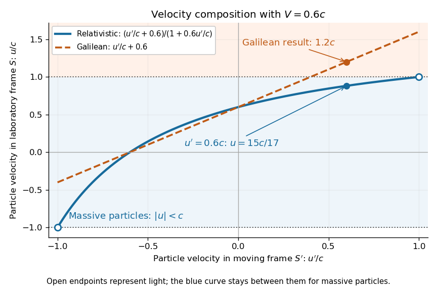
A short derivation differentiates the Lorentz transformation: $d{x}^{\prime }={\gamma }_V(dx-Vdt)$ and $d{t}^{\prime }={\gamma }_V(dt-Vdx/c^2)$. Dividing these differentials gives the longitudinal velocity-addition formula. The transverse formulas use $d{y}^{\prime }=dy$ and $d{z}^{\prime }=dz$, but the same transformed time denominator; omitting it would ignore the relativity of simultaneity. Replacing $V$ by $-V$ gives the inverse. When both relative and particle velocities are small compared with the speed of light, the denominator is close to one and the nonrelativistic limit recovers the Galilean transformation.

The formula lets us compare particle motion in a moving apparatus and a laboratory without losing the invariant speed of light. Einstein's 1905 paper derives the coordinate change in §3 and the composition of velocities in §5, including the collinear formula, its light-speed case, and composition of parallel transformations. ^[ref]. The rapidity parametrization makes the collinear composition particularly simple.

The velocity ellipsoid represents the positive velocity covariance tensor by its orthogonal principal axes and eigenvalue square roots. The uncentered second-moment tensor differs from covariance when a population streams. Vanishing mixed second moments align the second-moment ellipsoid with the chosen frame; for pure azimuthal streaming in a phase-mixed axisymmetric model, the off-diagonal covariance also vanishes.

A small planar velocity kick on a stellar circular orbit produces a local epicyclic motion in the source's rotating reference frame. With outward $x$, forward $y$, and initial displacements zero, Hill equations give $x/(\gamma a)=2\cos \theta (1-\cos nt)+\sin \theta \sin nt$ and $y/(\gamma a)=\cos \theta (4\sin nt-3nt)+2\sin \theta (\cos nt-1)$. Tangential kicks combine an epicycle with Keplerian shear; a radial kick gives a closed leading-order epicyclic ellipse.

For an instantaneous in-plane change of velocity of magnitude $\gamma v_K$ on a circular orbit, with angle $\theta$ measured from the forward tangential direction, the new specific orbital energy gives $a^{\prime }/a=(1-2\gamma \cos \theta -{\gamma }^2{)}^{-1}$. The specific angular momentum gives $e^{\prime 2}=1-(1-2\gamma \cos \theta -{\gamma }^2)(1+\gamma \cos \theta {)}^2$. The signed semi-major axis becomes negative for an unbound hyperbolic Kepler orbit.

When the weak force depends only on velocity, the phase average is a periodic total derivative and vanishes. The leading phase is constant, while the amplitude evolves according to the remaining average. The sign of that drift determines damping or growth and must be checked from the force, rather than inferred from its velocity dependence alone.

Use a velocity potential to reconstruct an irrotational flow from one scalar field. A velocity potential $\varphi (\mathbf{x},t)$ satisfiesIt has units ${\mathrm{m}}^2{\mathrm{s}}^{-1}$ and is unchanged as a description of the velocity field when any function of time alone is added. For twice continuously differentiable $\varphi$, the identity curl of a gradient proves zero vorticity. In incompressible flow, taking the divergence also gives ${\nabla }^2\varphi =0$, the Laplace equation. This turns a three-component velocity field into a single harmonic function with appropriate boundary conditions. ^[ref]

For uniform flow $\mathbf{u}=(U,0,0)$, take $\varphi =Ux$. With $U=2\mathrm{m}{\mathrm{s}}^{-1}$, the change from $x=0$ to $x=3\mathrm{m}$ is $\Delta \varphi =6{\mathrm{m}}^2{\mathrm{s}}^{-1}$. By the fundamental theorem for line integrals, the line integral of velocity between these points equals that change along any path in the domain; a closed curve gives zero circulation.

For the potential line vortex, choose a local angle branch in polar coordinates and set $\varphi =K\theta$. Then $u_r={\partial }_r\varphi =0$ and $u_{\theta }=r^{-1}{\partial }_{\theta }\varphi =K/r$. One counterclockwise turn changes the continued velocity potential by $2\pi K$, although the velocity field returns to its original value. With $K=1{\mathrm{m}}^2{\mathrm{s}}^{-1}$, this change is $2\pi {\mathrm{m}}^2{\mathrm{s}}^{-1}$, exactly the circulation. A full annulus therefore admits local angle branches and a multivalued velocity potential, but no global single-valued velocity potential when $K\ne 0$. Cutting the annulus along a radial line allows a single-valued angle branch on the remaining domain. The obstruction is path independence, not a failure of the local gradient formula.

A velocity profile records the variation of velocity across a spatial coordinate, for example $u(z)$ across a parallel viscous layer. Its derivative sets the tangential shear stress in a Newtonian fluid, while its integral gives the volume flux.