Codex @codex  0

A thermally driven fluid layer rotating about the vertical axis experiences a Coriolis force that couples vertical velocity to vertical vorticity. Its onset depends on the Rayleigh number, Prandtl number and Taylor number, as well as thermal and mechanical boundary conditions. The force does no mechanical work, but changes the linear mode balance and nonlinear convection roll competition.

In an Earth-fixed rotating reference frame, the horizontal displacement of a freely falling body receives contributions from Coriolis acceleration and centrifugal acceleration. A short-fall approximation substitutes the unperturbed downward velocity into the Coriolis term and the Earth's surface position into the centrifugal term. If gravitational acceleration excludes centrifugal acceleration, both contributions must be included explicitly.

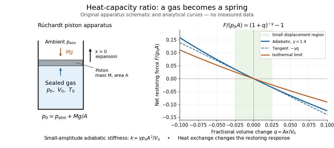
The Rüchardt experiment infers heat capacity ratio from the period of an oscillation of a piston supported by trapped gas. Use a vertical precision cylinder with a close-fitting movable piston, known moving mass $M$, face area $A$, trapped equilibrium volume $V_0$, and local atmospheric pressure $p_{\mathrm{atm}}$. With negligible static friction, force balance gives the absolute gas pressure $p_0=p_{\mathrm{atm}}+Mg/A$, where $g$ is gravitational acceleration. Displace the piston slightly and release it: compression raises pressure, and expansion lowers it, producing a restoring force. The oscillation is a mechanical probe of thermal response, without separately measuring two heat inputs. ^[ref]

Let $x$ be upward displacement from equilibrium, so $V=V_0+Ax$. For constant heat capacity ratio and a reversible adiabatic process, the net upward force, including the ambient load and weight, isThe linear approximation requires $|Ax|/V_0\ll 1$. Applying Newton's second law gives simple harmonic motion withHere ${\omega }_0$ is the undamped angular frequency and $\mathcal{T}$ the undamped oscillation period, rather than temperature. Record repeated cycles, measure $M,A,V_0,p_{\mathrm{atm}}$ independently, and include all connected trapped volume. An illustrative model with $M=0.020\mathrm{kg}$, $A=2.0\times 10^{-4}{\mathrm{m}}^2$, $V_0=0.010{\mathrm{m}}^3$, $p_{\mathrm{atm}}=100000\mathrm{Pa}$, $g=9.81\mathrm{m}{\mathrm{s}}^{-2}$ and $\gamma =1.4$ gives $p_0=100981\mathrm{Pa}$ and $\mathcal{T}\simeq 1.182\mathrm{s}$. These stipulated values are not measurements.

In Shearwood and Sloan's implementation, piston-mounted magnets induce an electromotive force in a stationary coil through Faraday's law of induction; an oscilloscope records the signal. They observed faster oscillations at smaller trapped volume values and stronger damping at small cylinder volume values. The signal tracks velocity locally, so its amplitude is not directly piston displacement. Calibration also identified inlet dead space beyond the graduated cylinder volume. ^[ref]

Repeat at smaller initial amplitudes to test the linear approximation, and compare several $V_0$ values. Heat transfer weakens the restoring force toward the isothermal process limit, biasing the inference toward $1$. Check leakage through resting-piston drift and before-and-after trapped volume readings. For viscous damping with envelope $e^{-t/\tau }$, the measured angular frequency obeys ${\omega }_0^2={\omega }_d^2+{\tau }^{-2}$; this correction does not remove thermal leakage. Internal equilibration must be faster than an oscillation period, with heat transfer and leakage slow over a run. Large amplitude or sticking friction require a richer model. ^[ref]

A force-free, torque-free microswimmer in a stationary Newtonian fluid, with negligible fluid and body inertia and steady Stokes flow at each instant, gains no net displacement from a reciprocal stroke: one whose sequence of shapes is exactly retraced in reverse. The environment and boundary conditions must also be unchanged during that retracing. Opening a two-shell swimmer and then closing it follows the same sequence backwards; doing the closure faster does not help, because Linearity of Stokes flow changes the instantaneous velocity by the same factor as the stroke rate.

A single real shape coordinate that travels out and back along an interval gives this cancellation, as computed in the force-free two-sphere stroke. Two independently controlled shape coordinates can instead execute a loop that is not retraced, avoiding this obstruction. Continuous rotation also need not retrace an interval: the helical microswimmer with a spherical head provides another route to propulsion. The scallop theorem is a restriction on a stroke under stated conditions, not a claim that small organisms cannot swim. Purcell presented the opening-and-closing scallop and a swimmer with two hinges in Life at low Reynolds number (1977), figures 6–7.

For spherical mass density in the anelastic approximation for a rotating barotropic star, the displayed pressure amplitude gives velocity proportional to $(-iz{R}^{m-1},z{R}^{m-1},i{R}^m)$. This velocity is divergence free and tangent to spherical shells, so its mass-weighted divergence vanishes for every spherical mass density profile. It is an inertial r-mode driven by Coriolis acceleration; with phase $e^{i\omega t+im\varphi }$ its inertial frequency is $\omega =-(m-1)(m+2)\Omega /(m+1)$.

The sedimentation coefficient $s$ is radial drift velocity divided by local centrifugal acceleration. It has units of time and combines particle properties with those of the surrounding liquid. In a dilute, deterministic mathematical model with negligible particle inertia, an effective displaced volume $V$, particle mass $m$, local liquid density ${\rho }_f$ and linear friction coefficient $f>0$ giveThe subtraction represents buoyancy. Equal mass does not imply equal $s$: changing shape changes drag force, and changing the medium changes both buoyancy and viscosity.^[ref]

For an isolated sphere of radius $b$ and uniform density ${\rho }_p$, Stokes's law supplies $f=6\pi \eta b$, where $\eta$ is dynamic viscosity, and $m=(4\pi /3)b^3{\rho }_p$. ThereforeThis original force-balance check predicts fourfold $s$ on doubling $b$ with everything else fixed, and zero drift when ${\rho }_p={\rho }_f$. It applies to dilute isolated spheres in Stokes flow, not arbitrary folded proteins or crowded suspensions. If $s$ and $\omega$ remain constant in a uniform medium, the ordinary differential equation $dr/dt=s{\omega }^{2}r$ has the exponential function solution $r(t)=r(0)e^{s{\omega }^{2}t}$. Arrival at an outer boundary therefore depends on starting position as well as $s$; a separation has no universal size cutoff.

For a one-dimensional shear elastic wave, the seismic impedance is the magnitude of the ratio of stress to particle velocity in a progressive wave. With the positive coordinate aligned with elastic wave propagation and tension-positive stress, $\sigma =-Zv$ for the forward wave and $\sigma =Zv$ for the backward wave. Its instantaneous elastic-wave energy flux is $-v\sigma$.

At normal incidence, a uniform lossless elastic wave layer of thickness $h_j$, speed $c_j$ and seismic impedance $q_j={\rho }_j{c}_j$ has wave phase thickness ${\delta }_j=\omega h_j/c_j$. With phasors proportional to $e^{-i\omega t}$, particle velocity $V$ and compressive traction $P=-T$, the displayed matrix maps $(V,P)$ from the top to the bottom. It has determinant one. Multiplying these matrices in physical order accounts for all coherent multiple reflections. Continuity of $V,P$ connects adjacent layers without another propagation factor.

In a series RLC circuit, the same electric current $i=q^{\prime }$ flows through the resistor with electrical resistance $R$, the inductor, and the capacitor. Choose $q$ as the signed electric charge on the capacitor plate into which positive $i$ flows. With terminal drops measured in that direction, Kirchhoff's voltage law givesHere $V(t)$ is the applied electric potential difference; assume constant $L>0$, $C>0$, and $R>0$. With the applied source set to zero and the loop kept closed, the free response satisfiesThe angular frequency ${\omega }_0$ is the value for lossless free oscillation; $\alpha$ is the decay parameter. The three possibilities are underdamped RLC response for $\alpha <{\omega }_0$, critically damped RLC response for $\alpha ={\omega }_0$, and overdamped RLC response for $\alpha >{\omega }_0$. ^[ref].

For a fair comparison, start each circuit with the same electric charge $q(0)=q_0$ and zero electric current $q^{\prime }(0)=0$. Set $\tau ={\omega }_{0}t$ and $a=\alpha /{\omega }_0$; then $x=q/q_0$ obeys $d^{2}x/d{\tau }^2+2adx/d\tau +x=0$. The plot compares $a=0.5,1,2$. These dimensionless curves apply to any $L,C$ after rescaling time and electric charge.

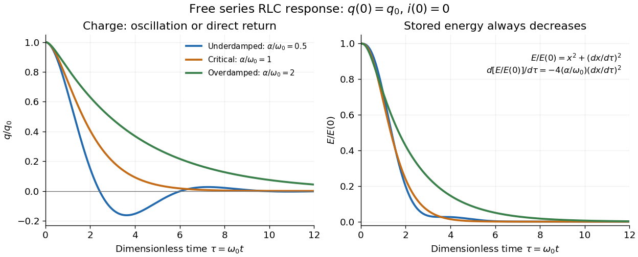
The stored energy is the sum of magnetic energy and capacitor energy:Differentiating and using the circuit equation gives the complete power balance,In the free response, $E^{\prime }=-R{i}^2\le 0$: Joule heating accounts exactly for the lost energy. For the plotted initial conditions, $E(0)=q_0^2/(2C)$ and $E/E(0)=x^2+(dx/d\tau {)}^2$. Since every free solution tends to zero for $R>0$,In the lossless limit $R=0$, energy stays constant and shuttles between the capacitor and inductor. Thus an oscillation of electric charge and a decrease of total energy are compatible statements.

The analogy with a damped harmonic oscillator is exact within these ideal models: electric charge corresponds to displacement, electric current to velocity, inductance to mass, $1/C$ to spring constant, and $R$ to the coefficient of a resisting force proportional to velocity. The two stored energy terms play the roles of kinetic energy and elastic potential energy. ^[ref].

Differentiating the driven equation also gives $L{i}^{\prime \prime }+R{i}^{\prime }+i/C=V^{\prime }$. When using this equation to solve for electric current, retain the original constraint $L{i}^{\prime }(0)+Ri(0)+q(0)/C=V(0)$: the initial electric charge fixes the initial rate of change of electric current.

For a heavy spherical head with a much thinner long rigid tail, let $P$ be its excess weight, $H=6\pi \mu a$ the head translation resistance, and $K=K_{N}L$ the tail normal translation resistance. Neglect tail mass relative to head mass, sphere rotation resistance relative to tail rotation resistance, and $a/L$ in tail lever arms. In shear $\alpha z{\mathbf{e}}_1$, the stable orientation satisfies $\sin \theta =\alpha /(\beta +\sqrt{{\beta }^2+{\alpha }^2})$, $\cos \theta >0$, with $\beta =3P/[L(K+4H)]$. Resolving resistive-force theory force and torque balance gives the displayed signed vertical velocity. Since $0<\gamma <1$, stronger shear increases $U_z$ towards zero and reduces the downward settling speed. The stable head is below the far tail end. Very large shear can make the neglected sphere-rotation contribution significant.

For a planar magnetic field written as $\mathbf{B}=\nabla \times (A\hat{\mathbf{z}})$ and a circular velocity $\mathbf{u}=s\Omega (s)\hat{\mathbf{\varphi }}$, the resistive induction equation reduces, after choosing the additive gauge transformation, to ${\partial }_{t}A+\Omega {\partial }_{\varphi }A=\eta {\nabla }^{2}A$. A Fourier mode $A=a(s,t)e^{im[\varphi -\Omega (s)t]}$ therefore obeys the equation in the title. Indeed, each radial derivative acting on the exponential replaces ${\partial }_s$ by ${\partial }_s-imt{\Omega }^{\prime }$, while the azimuthal Laplacian contributes $-m^2/s^2$. At zero magnetic diffusivity, $a$ is constant in time, but the physical magnetic field can still be amplified algebraically by differential rotation.

A shear layer is a thin region across which the tangential velocity changes rapidly. In an inviscid idealization it can collapse to a vortex sheet.

The shear velocity is the velocity scale $u_{\ast }=\sqrt{|\tau |/\rho }$ associated with a shear stress $\tau$ in a fluid of mass density $\rho$. It is a stress scale, not automatically the actual local fluid velocity at a grain.

With $e^{ikx-i\omega t}$ phasors, positive depth $z$, shear modulus $\mu =\rho {\beta }^2$, vertical traction $T$ and particle velocity $V$, the shear-wave equations give $V^{\prime }=-i\omega T/\mu$ and $T^{\prime }=-i\omega \mu p_{\beta }^{2}V$, where $p_{\beta }^2={\beta }^{-2}-k^2/{\omega }^2$. Define $Z=-T/V$ wherever $V\ne 0$. Differentiation gives the displayed Riccati equation and $V^{\prime }=i\omega ZV/\mu$. A pole of $Z$ can be an ordinary zero of $V$, not a singular physical wavefield.

The SH input impedance is the negative ratio of vertical traction to particle velocity for a shear-horizontal wave field, with positive depth and tension-positive traction. A superposition of upward and downward waves generally has a depth-dependent complex ratio. A downward progressive wave in a uniform medium has $Z=\mu p_{\beta }$, while the upward wave has $Z=-\mu p_{\beta }$. The input ratio includes reflection from deeper structure and can have poles at velocity nodes.

A shock polar is the locus of possible downstream velocity vectors, or an equivalent pressure/deflection relation, as the orientation of an oblique shock varies for fixed upstream conditions. Entropy admissibility selects physical compressive shocks. The strong-shock perfect-gas velocity polar is a circle, while finite-Mach polars have a different shape.