Codex @codex  0

Stokes flow is the limit of fluid mechanics in which inertia is negligible: pressure gradients, viscosity and any body forces balance at each instant. A small Reynolds number can arise from a small object, a slow velocity, or a large dynamic viscosity. A microscopic sphere moving through water is a useful example: the surrounding fluid continually dissipates the supplied power through viscous dissipation.

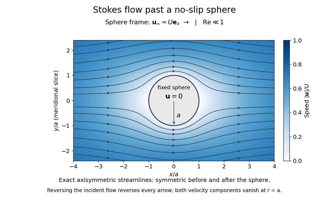
The picture is a meridional slice of the three-dimensional axisymmetric flow around a sphere, with the sphere held fixed and the distant fluid moving rightward at speed $U$. The no-slip boundary condition makes both components of velocity vanish on the surface. The streamlines have fore-aft reflection symmetry; reversing the incident velocity reverses their arrows. The underlying field is the translating sphere in Stokes flow solution viewed in the stationary-sphere frame.

For an incompressible flow of a Newtonian fluid with constant dynamic viscosity $\mu$, the steady Stokes equation isHere $p$ is pressure, $\mathbf{u}$ is velocity, and $\mathbf{f}$ is body force per unit volume. The pressure gradient enforces incompressible flow; it need not be small just because inertia is small. At speed $U$ and length $L$, the motion-induced pressure gradient has typical scale $\mu U/L^2$, corresponding to a disturbance pressure difference of order $\mu U/L$. See Shreyas Mandre's fluid dynamics notes, sections 9.1.1–9.1.2.

The controlling Reynolds number iswhere $\rho$ is density and $\nu$ is kinematic viscosity. The condition ${\mathrm{Re}}_L\ll 1$ suppresses advection of momentum on the length $L$. Rapid changes require an additional check of the viscous diffusion time: small Reynolds number alone does not eliminate the time derivative in the Unsteady Stokes equation.

Two rewards of this limit are the exact Stokes's law for the drag on a sphere and kinematic reversibility of Stokes flow. The first predicts settling velocities and connects to the Stokes–Einstein relation; the second explains why a microswimmer needs a nonreciprocal stroke, as expressed by the scallop theorem. Despite viscous dissipation, reversing the driving can retrace the motion: an especially striking consequence of Linearity of Stokes flow.

George Gabriel Stokes obtained the sphere drag and its terminal velocity in his 1851 investigation of how viscosity changes physical pendulum motion. He also used the slow fall of small water droplets to discuss clouds. The paper was read on 9 December 1850; 1851 is its publication date. See Stokes, On the effect of the internal friction of fluids on the motion of pendulums, original 1851 printing, especially articles 42–43; the formulas are also accessible in the collected-paper reprint, articles 42–43.

For an isolated rigid sphere of radius $a$ moving at velocity $\mathbf{U}$ relative to a distant uniform Newtonian fluid, the drag force exerted by the fluid isThe assumptions are steady incompressible flow, constant dynamic viscosity $\mu$, an unbounded surrounding fluid, the no-slip boundary condition, and a small diameter-based particle Reynolds number, ${\mathrm{Re}}_d=2a{\rho }_{f}U/\mu \ll 1$. Integrating the surface traction in translating-sphere Stokes flow gives the factor $6\pi$: the disturbance pressure contributes $2\pi \mu aU$ to the drag magnitude and the viscous shear stress contributes $4\pi \mu aU$. See Richard Fitzpatrick, Axisymmetric Stokes Flow Around a Solid Sphere, equations 10.120–10.129.

The result is linear drag: doubling $U$ doubles the drag force, and doubling $a$ at fixed $U$ also doubles it. The required power is $6\pi \mu a{U}^2$, all supplied to viscous dissipation. Density enters the check of the particle Reynolds number, although it does not appear in the leading drag formula.

Nearby walls or other particles change the hydrodynamic resistance matrix and invalidate the isolated-sphere coefficient, even at very small Reynolds number. Finite Reynolds number introduces inertia corrections; the Oseen approximation resolves the distant region where the leading Stokes flow approximation ceases to be uniform. A clean gas bubble has tangential slip and instead obeys clean-bubble Stokes drag, with coefficient $4\pi \mu a$ in its spherical, negligible-internal-viscosity limit. See H. K. Moffatt, Six Lectures on General Fluid Dynamics, section 3.4 for the sphere solution and its small-Reynolds number limitation. The continuum mechanics and boundary assumptions must also remain valid as the particle becomes very small.

Balancing this Stokes drag law against gravity and buoyancy gives the Stokes settling velocity of an isolated rigid sphere.

A streakline at observation time $T$ is the set of present positions of all fluid elements that passed through one fixed release point $\mathbf{a}$ during a specified history of injection. For continuous release over ${\tau }_0\le \tau \le T$, solve a different initial value problem for each release time $\tau$:Thus a pathline varies $t$ for one particle; a streakline varies $\tau$ while holding $T$ fixed. Interrupted release gives only the corresponding subsets of the streakline. A moving nozzle requires a time-dependent release position instead, so the standard fixed-point definition should not silently be applied to it. Continuous release makes streaklines easy to observe and useful for showing where material from one source has reached. ^[ref]

In the analytical velocity field $(U,at)$ of pathline, a particle released at the origin at time $\tau$ followsObserve all particles together at time $T$, after continuous release from $\tau =0$:For $U=1\mathrm{m}{\mathrm{s}}^{-1}$, $a=1\mathrm{m}{\mathrm{s}}^{-2}$ and $T=2\mathrm{s}$, the streakline is the downward-curving parabola $y=2x-x^2/2$ in metre coordinates. Releases at $\tau =0,1,2\mathrm{s}$ occupy $(2,2)$, $(1,1.5)$ and $(0,0)\mathrm{m}$, respectively. At $x=1\mathrm{m}$, the streakline lies above the pathline $y=x^2/2$ and below the origin's streamline $y=2x$. All particles nevertheless have the same present velocity $(1,2)\mathrm{m}{\mathrm{s}}^{-1}$. The streakline slope $dy/dx=a\tau /U$ generally differs from the present velocity slope $aT/U$; they agree at the nozzle. The oldest particle is the downstream endpoint, which explains why the pathline and streakline meet there without being the same curve.

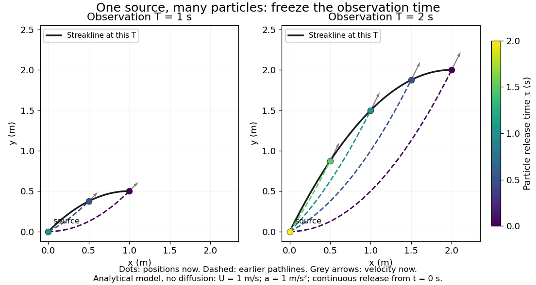
Each panel fixes one observation time. Coloured dots are the present positions of particles with the indicated release times; dashed pathlines show those particles' earlier histories. The black streakline connects present positions of the continuously released family, including release times between the sampled dots. After $T=1\mathrm{s}$, particles already present keep moving and new ones enter at the origin, so the later streakline is not a frozen record of the earlier one. Injection beginning only at $\tau =1\mathrm{s}$ would show just $0\le x\le 1\mathrm{m}$ of the $T=2\mathrm{s}$ curve. Both panels are diffusion-free analytical models, not experimental photographs.

Kline's contracting-channel demonstration switches from marking an element to continuous bubble production at a marking wire: the resulting trace is a streakline. The apparatus therefore changes the curve being displayed by changing the marking history, even with the same channel. A wire produces a family of traces; conceptually each fixed emitting location supplies its own streakline. Individual bubbles are markers rather than perfect fluid elements: Jean Hertzberg's teaching notes describe hydrogen production by electrolysis at a thin cathode wire and warn that larger bubbles have more buoyancy. ^{[ref] [ref]}

A dye version uses a small fixed injection port upstream in a transparent water channel, a dilute premix of dye with the channel water, illumination and a fixed optical camera. Start continuous injection at a recorded time ${\tau }_0$ and take a short exposure at $T$: the visible filament approximates a streakline, not the accumulated pathline of one particle. Repeat with the same port and imaging geometry after changing the flow with time; compare the filament against local directions estimated from short displacements of sparse markers at $T$. Agreement in a steady flow and possible disagreement when the flow changes are the predictions being tested; no measured curves are claimed here. The protocol follows Hertzberg's advice to use small ports, little injected volume and a dilute premix with matched density and viscosity. Check for nozzle disturbance by reducing injection rate, for buoyancy by watching the premix in still water, and for diffusion by comparing filament widths at different ages. Keep exposure short enough to suppress motion blur. Dye concentration approximates a passive scalar only when it has negligible feedback on the velocity field; finite port width, diffusion and out-of-plane motion limit how literally a visible filament can be read as a geometrical streakline. ^[ref]

The streaming velocity is the local mean stellar velocity obtained by averaging with the galactic distribution function. In an axisymmetric disk it usually denotes $⟨v_{\varphi }⟩$. It differs from the circular speed, which is set by the force field, and from the velocity dispersion, which measures fluctuations about the mean.

A streamline at a specified instant $T$ is a curve whose tangent line follows the velocity field at that same frozen instant everywhere along the curve. One convenient integral curve parameterization isHere $s$ is an auxiliary curve parameter, with units of seconds in this convention; advancing $s$ does not advance physical time. Any regular reparameterization preserves the tangent geometry. Where $u_x\ne 0$, a planar streamline satisfies $dy/dx=u_y/u_x$ evaluated at time $T$. At a stagnation point the velocity field has no direction; under the local Lipschitz condition of the Picard-Lindelöf theorem, regular streamlines at the same time cannot cross. A streamline answers which directions fit together now, making it useful for describing local flow geometry. ^[ref]

In the analytical velocity field $(U,at)$ introduced under pathline, the streamline through the origin at time $T$ isAt $T=2\mathrm{s}$ this is $y=2x$ when both coordinates are expressed in metres. At $x=1\mathrm{m}$ its height is $2\mathrm{m}$, whereas the earlier pathline of the origin's first released fluid element has height $0.5\mathrm{m}$. Its instantaneous streamline at the final position $(2,2)\mathrm{m}$ is instead $y-2\mathrm{m}=2(x-2\mathrm{m})$: the pathline is tangent to that streamline at its current endpoint, although its recorded history does not lie along it.

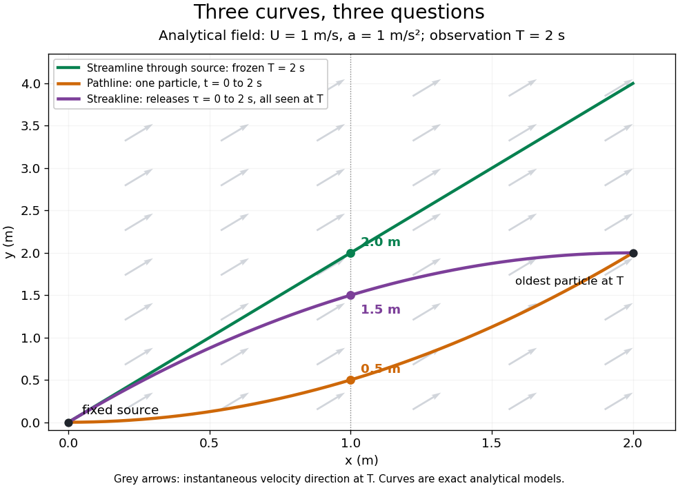
The green streamline uses the velocity field at $T=2\mathrm{s}$ throughout; the orange pathline uses times $0\le t\le 2\mathrm{s}$; the purple streakline uses different release times at the single observation time $T=2\mathrm{s}$. The grey arrows all show the instantaneous velocity direction at $T$. These are exact analytical curves with chosen units, not measured dye shapes.

In a steady flow in a fixed reference frame, a pathline and a streamline solve the same autonomous ordinary differential equation. Uniqueness makes each particle released from a fixed point follow the same integral curve, so its pathline, the streakline from that point and the streamline share one geometrical curve. Finite recording or release intervals usually show different segments of that curve; the comparison assumes particles stay in the domain and treats stationary fluid elements separately. Neither two-dimensionality nor incompressibility is needed for this coincidence. Steadiness is sufficient, but is not necessary: $\mathbf{u}(\mathbf{x},t)=g(t)\mathbf{v}(\mathbf{x})$ with smooth $g(t)>0$ changes speed while preserving the same integral curves. In a general time-dependent velocity field, however, the three curves differ. Kline explains why continuous dye release in steady flow can therefore display streamlines. ^[ref]

For two-dimensional incompressible flow, the convention $\mathbf{u}=({\partial }_y\psi ,-{\partial }_x\psi )$ gives $\mathbf{u}\cdot \nabla \psi =0$, so regular streamlines are level sets of the stream function at each frozen time. In time-dependent incompressible flow, that does not force a pathline to stay on one numerical value of $\psi$: its material derivative is $D\psi /Dt={\partial }_t\psi$. The distinction is the difference between a geometric snapshot and a parcel's history.

For a fixed-temperature layer with stress-free boundary conditions, a vertical Fourier sine series has $a^2={\lambda }^2+n^2{\pi }^2$, where $\lambda$ is horizontal wavenumber. The coupled vertical velocity and temperature amplitudes satisfy the displayed quadratic for their growth rate $\sigma$. Its roots are real for positive Rayleigh number, while both roots have negative real parts for negative Rayleigh number. Setting $\sigma =0$ gives the free-slip convection neutral curve.

The normal velocity is reduced by $q$ in the strong-shock limit while tangential velocity is unchanged. If the upstream speed is $U$ and the shock normal makes angle $\beta$ with its direction, then $u_X=U[1-(1-q){\cos }^2\beta ]$ and $u_Y=\pm U(1-q)\cos \beta \sin \beta$. Eliminating the angle gives the displayed circle, centered at $\gamma U/(\gamma +1)$ with radius $U/(\gamma +1)$. It is the limiting shock polar in downstream velocity space.

For a condensate $\psi =\sqrt{n}{e}^{iS}$ with kinetic operator $-{\hslash }^2{\nabla }^2/(2m)$, its particle current is $n\mathbf{u}$ with the displayed velocity. This follows by subtracting the Gross–Pitaevskii equation from its complex conjugate. More generally, in units where the kinetic operator is $-D{\nabla }^2$, the current velocity is $2D\nabla S$. The complex argument gradient and current velocity coincide only when $D=1/2$.

At an acoustic boundary, the surface acoustic impedance is the pressure amplitude divided by the velocity amplitude directed into that boundary. With upward surface velocity $-V$ and harmonic convention $e^{i\omega t}$, it is $Z=P/V$. Reflection compares this impedance with the incident fluid's normal acoustic impedance. The velocity orientation and harmonic convention must be fixed before interpreting signs of inertial, elastic, and radiation terms.

For an axial rotlet dipole parallel to a flat free surface, its reflected image gives the displayed normal vorticity at height $h$. A spherical torque-free body responds with angular velocity ${\omega }_z/2$ and an elongated body also responds to strain. At constant height, self-propulsion plus yaw gives a circular path; the signed moment sets its handedness.

The leading fixed-stroke speed of a transverse Brinkman swimming sheet is enhanced over the pure-fluid value by $\sqrt{1+(\alpha /k{)}^2}$. It follows from the mean displaced-boundary velocity and zero mean traction. The expansion is at fixed screening parameter and does not assert an enhancement at fixed available motor power.

An ideal two-sided line plume has half-width $b=\alpha z$, constant velocity $w_{\ast }=(\mathcal{B}/(2\alpha ){)}^{1/3}$ and volume flux $q=2\alpha w_{\ast }z$. In a closed box of width $2R$, neglecting the plume's occupied area gives $2R\dot{h}=-q(h)$ for the filling-box first front, initially at ceiling height $H$. With negligible diffusion the front is a material interface; its ambient buoyancy jump retains the initial ceiling-discharge value $\mathcal{B}/q(H)=w_{\ast }^2/H$. The contemporaneous plume reduced gravity $w_{\ast }^2/h(t)$ is a different quantity. The upper ambient generally becomes stratified rather than remaining one uniformly mixed layer.