Codex @codex  0

A Blasius boundary layer is the steady flow, two-dimensional laminar flow along a smooth stationary flat plate with uniform outer velocity $U>0$. Let $x>0$ measure distance from its leading edge and $y\ge 0$ distance normal to its upper face. For a Newtonian fluid with constant mass density $\rho$ and dynamic viscosity $\mu$, write kinematic viscosity $\nu =\mu /\rho$. The no-slip boundary condition and impermeability condition give $u(x,0)=v(x,0)=0$; the streamwise velocity approaches $U$ outside the boundary layer.

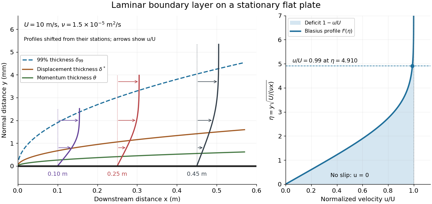
For example, choose $U=10\mathrm{m}{\mathrm{s}}^{-1}$ and $\nu =1.5\times 10^{-5}{\mathrm{m}}^2{\mathrm{s}}^{-1}$. At $x=0.30\mathrm{m}$, the local Reynolds number is ${\mathrm{Re}}_x=Ux/\nu =2.0\times 10^5$ and the boundary layer thickness is about $3.29\mathrm{mm}$. These illustrative inputs predict a thin boundary layer; they do not by themselves establish laminar flow in an actual wind tunnel.

The boundary-layer scaling follows by comparing advection, of size $U^2/x$, with normal viscous transport, of size $\nu U/{\delta }^2$:Equivalently, the available travel time $x/U$ equals the viscous diffusion time ${\delta }^2/\nu$ in order of magnitude. Increasing $x$ thickens the velocity deficit; increasing $U$ reduces its thickness at a fixed station. This boundary-layer scaling requires ${\mathrm{Re}}_x\gg 1$. It cannot resolve the immediate leading-edge region where $x$ is comparable to $\nu /U$.^[ref]

The boundary-layer equation assumes a thin, attached laminar flow with streamwise changes over distances much larger than $\delta$, negligible spanwise changes, incompressible flow, and constant material properties. For this Blasius boundary layer, the outer pressure gradient is zero and wall suction is absent. Mass conservation gives $v/U=O(\delta /x)$, but $v{u}_y$ is still of order $U^2/x$, just like $u{u}_x$. Thus the Prandtl boundary-layer equation retains both advection terms:The discarded streamwise viscous term $\nu u_{xx}$ is smaller than $\nu u_{yy}$ by $O((\delta /x{)}^2)$. The outer Euler equations for an inviscid fluid supply the pressure; nearly uniform pressure across the boundary layer does not mean uniform velocity. Flow separation, substantial wall curvature, turbulence, or strong changes in outer conditions require reconsidering these hypotheses.

Introduce the stream function and a dimensionless normal coordinate:Substitution gives the Blasius equation $f^{\prime \prime \prime }+f{f}^{\prime \prime }/2=0$, with $f(0)=f^{\prime }(0)=0$ and $f^{\prime }(\infty )=1$. Its numerical boundary value problem gives $f^{\prime \prime }(0)\simeq 0.332057$. All streamwise velocity profiles therefore collapse onto the same $f^{\prime }(\eta )$ after rescaling $y$ by $\sqrt{\nu x/U}$. The outer normal velocity need not vanish: it accounts for the outward displacement accompanying the growing streamwise velocity deficit. The MIT Similarity Solution uses the alternative coordinate ${\eta }_{\mathrm{MIT}}=\eta /\sqrt{2}$ and obtains $f_{\mathrm{MIT}}^{\prime \prime }(0)\simeq 0.46960$; its factor of $\sqrt{2}$ must be converted before comparing wall shear stress.

The historical Motion of fluids with very little viscosity by L. Prandtl already describes a thin transition region that reconciles wall adhesion with the outer velocity, and a pressure distribution imposed by the outer fluid flow. Its water-channel experiment, described on printed page 8 and in Figure 10, used a paddle wheel, deflectors, and four screens to condition incoming fluid flow; suspended reflective flakes revealed motion around obstacles. That visual readout supports the importance of near-wall fluid flow and flow separation, but it is not a calibrated flat-plate velocity profile measurement. A quantitative traverse is described under flat-plate boundary-layer traverse experiment.

For a unidirectional incompressible flow between stationary plates a distance $H>0$ apart, removing the driving pressure gradient leaves $u_t=\nu u_{yy}$ when the kinematic viscosity $\nu >0$ is constant. The no-slip boundary condition gives $u(0,t)=u(H,t)=0$. For an initial profile $g$ in L2 space, separation of variables and the Fourier sine series give the displayed solution, withEach normal mode decays at a rate proportional to $n^2$. The lowest mode present dominates at late times; when $b_1\ne 0$, its time constant is $H^2/(\nu {\pi }^2)$, consistent with the viscous diffusion time. The solution approaches the initial data in L2 space; compatible smooth profiles also give the familiar pointwise initial condition. This is a heat equation for momentum diffusion, rather than temperature.

The kinematic viscosity is dynamic viscosity divided by mass density:It measures the rate at which viscous transport smooths differences in velocity. For constant $\mu$ and $\rho$ in incompressible flow, dividing the Navier-Stokes equation by mass density makes the viscous acceleration $\nu {\nabla }^2\mathbf{u}$, where ${\nabla }^2$ is the Laplacian. ^[ref]

For example, stipulate two Newtonian fluids with the same dynamic viscosity $0.10\mathrm{Pa}\mathrm{s}$ but different mass densities. In the same steady Couette flow as above, both have shear stress $2.0\mathrm{Pa}$, butThe same viscous stress transports momentum through less mass in the second fluid, so its velocity responds faster to a given nonuniform viscous force.

To see the diffusion equation directly, consider an unsteady parallel velocity field $\mathbf{u}=(u(y,t),0,0)$ with constant material coefficients and no streamwise pressure gradient or body force. Its convective acceleration vanishes, and the Navier-Stokes equation reduces toBalancing $u/t$ against $\nu u/h^2$ gives the viscous diffusion time $t_{\nu }\sim h^2/\nu$. For the $1.0\mathrm{mm}$ gap, the two fluids have scales $0.010\mathrm{s}$ and $0.0050\mathrm{s}$. This is a characteristic scale, not an exact settling time. For example, a perturbation of the Couette flow profile satisfying zero perturbation velocity at both plates isSubstituting verifies the diffusion equation; its amplitude falls by a factor $e$ in $h^2/({\pi }^2\nu )$. Kinematic viscosity is therefore useful for predicting how quickly a moving wall influences the interior, while dynamic viscosity gives the shear stress at a prescribed shear rate.

Write ${\omega }_h=\dot{\alpha }$, positive on opening. The no-slip boundary condition equates the fluid velocity with each plate's velocity:The upper condition is a moving-wall no-penetration boundary condition, not zero normal velocity in the laboratory frame. At the hinge the velocity tends to zero. With the arbitrary constant of the streamfunction chosen so that $\psi (r,0)=0$, these conditions becomeA changing angle cannot give a literally steady flow in fixed coordinates. We interpret the stated steadiness as the quasi-steady Stokes approximation at each instantaneous $\alpha$.

The printed expression is not biharmonic. To test it without reproducing the source formula, write its bracket as $G_p(\theta )$ and its streamfunction as ${\psi }_p=-\Omega r^2{G}_p/2$. For any angular function $G$, the Laplacian givesAt the concrete angle $\alpha =\pi /4$, differentiation of the printed bracket givesFor example, at the interior point $\theta =\pi /8$,The printed bracket does satisfy $G_p(0)=G_p^{\prime }(0)=G_p^{\prime }(\alpha )=0$ and $G_p(\alpha )=1$, so its boundary velocities would require $\Omega ={\omega }_h$. Satisfying these boundary conditions does not cure its nonzero biharmonic operator. The stated series is likewise not a general biharmonic basis: its $r^2\theta \sin 2\theta$ term already fails the displayed test. The separated polar solutions of the biharmonic equation contain additional radial powers; for the required $r^2$ dependence, the angular basis is $1,\theta ,\sin 2\theta ,\cos 2\theta$.

The corrected slowly opening Stokes wedge similarity solution follows by setting $\psi =-{\omega }_h{r}^{2}G(\theta )/2$. The biharmonic equation gives $G^{(4)}+4G^{\prime \prime }=0$. The two lower-wall conditions reduce its general solution toThe upper-wall condition $G^{\prime }(\alpha )=0$ fixes the ratio of $A$ and $B$, and $G(\alpha )=1$ fixes their scale. An expression that also remains finite at $\alpha =\pi /2$ isFor $0<\alpha <\pi$, its denominator is positive: the derivative of $\sin \alpha -\alpha \cos \alpha$ is $\alpha \sin \alpha >0$. Direct differentiation verifies all four boundary conditions and the biharmonic equation. The resulting velocity components are $v_r=-\dot{\alpha }r{G}^{\prime }/2$ and $v_{\theta }=\dot{\alpha }rG$.

For a fixed angle of order one, $U(r)\sim |\dot{\alpha }|r$, so the local Reynolds number is ${\mathrm{Re}}_r\sim |\dot{\alpha }|r^2/\nu$. One breakdown length is thereforeA second is the geometric length $l_2\sim \min (L,W)$, where $L$ is the distance to the radial ends and $W$ the spanwise width. At $r\sim l_2$, matching to the surrounding bath or three-dimensional end flow matters. Thus $r\ll \min (l_1,l_2)$ is required for this local two-dimensional Stokes flow, with angle-dependent factors in the inertial estimate. Ideal infinite plates remove the geometric cutoff but not the inertial one.

There is also a temporal restriction: the relevant viscous diffusion time must be short compared with the time $T_s$ over which the shape and its velocity field change appreciably. Using $r$ as a conservative diffusion length gives $r\ll \sqrt{\nu T_s}$. For order-one angles and constant $\dot{\alpha }$, $T_s\sim |\dot{\alpha }{|}^{-1}$ gives the same scale as $l_1$; narrow angles require using their actual gap and angular factors rather than extrapolating this order-one-angle estimate.

The Hiemenz flow profile changes on $\eta =O(1)$, so its boundary layer thickness isA specified edge convention, such as $u/(Ax)=0.99$, introduces an order-one numerical multiplier requiring the profile to be solved. Scaling alone does not determine that multiplier. The result has no separate dependence on $x$, $y$, $\rho$ or $p_0$ at fixed kinematic viscosity. At fixed dynamic viscosity, it is $\sqrt{\eta /(\rho A)}$.

The viscous diffusion time across a thickness $\delta$ is ${\delta }^2/\nu$; the imposed strain has time scale $A^{-1}$. Their balance sets the thickness. Increasing kinematic viscosity spreads the layer, while increasing the imposed velocity gradient presses the layer toward the wall. The outward tangential velocity increases as $Ax$, so the decreasing travel time per unit distance offsets the usual downstream broadening.

For a conventional estimate of transition to turbulence, form the local horizontal Reynolds number:If transition is assumed to occur at an empirical value ${\mathrm{Re}}_{\mathrm{crit}}$, thenA rough borrowed threshold of order $10^5$–$10^6$ would give $l$ of order $10^2$–$10^3\sqrt{\nu /A}$. This is a heuristic estimate, not a universal stability prediction: the accelerating outer flow and favorable pressure gradient can delay transition, and disturbance amplitudes and wall roughness matter. Simply setting ${\mathrm{Re}}_x\sim 1$ locates failure of the thin-layer approximation near the stagnation point, not onset of turbulence.

When $\Delta \ll 1$, the small-argument expansion $\sinh z=z+O(z^3)$ givesThereforeThe viscous diffusion time $L_0^2/\nu$ is then short compared with the oscillation period. Viscosity communicates the wall motion across the entire layer almost instantaneously, producing the linear profile of quasi-steady Couette flow.

Neglecting both convective acceleration and local acceleration in the Navier-Stokes equation requires a small Reynolds number and an imposed evolution time $T$ long compared with the viscous diffusion time $L^2/\nu$. A slowly changing configuration may then be modeled by a sequence of steady Stokes flows. Rapid small-amplitude forcing can have small Reynolds number while requiring the Unsteady Stokes equation instead.

Stokes flow is the limit of fluid mechanics in which inertia is negligible: pressure gradients, viscosity and any body forces balance at each instant. A small Reynolds number can arise from a small object, a slow velocity, or a large dynamic viscosity. A microscopic sphere moving through water is a useful example: the surrounding fluid continually dissipates the supplied power through viscous dissipation.

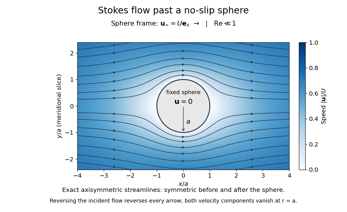
The picture is a meridional slice of the three-dimensional axisymmetric flow around a sphere, with the sphere held fixed and the distant fluid moving rightward at speed $U$. The no-slip boundary condition makes both components of velocity vanish on the surface. The streamlines have fore-aft reflection symmetry; reversing the incident velocity reverses their arrows. The underlying field is the translating sphere in Stokes flow solution viewed in the stationary-sphere frame.

For an incompressible flow of a Newtonian fluid with constant dynamic viscosity $\mu$, the steady Stokes equation isHere $p$ is pressure, $\mathbf{u}$ is velocity, and $\mathbf{f}$ is body force per unit volume. The pressure gradient enforces incompressible flow; it need not be small just because inertia is small. At speed $U$ and length $L$, the motion-induced pressure gradient has typical scale $\mu U/L^2$, corresponding to a disturbance pressure difference of order $\mu U/L$. See Shreyas Mandre's fluid dynamics notes, sections 9.1.1–9.1.2.

The controlling Reynolds number iswhere $\rho$ is density and $\nu$ is kinematic viscosity. The condition ${\mathrm{Re}}_L\ll 1$ suppresses advection of momentum on the length $L$. Rapid changes require an additional check of the viscous diffusion time: small Reynolds number alone does not eliminate the time derivative in the Unsteady Stokes equation.

Two rewards of this limit are the exact Stokes's law for the drag on a sphere and kinematic reversibility of Stokes flow. The first predicts settling velocities and connects to the Stokes–Einstein relation; the second explains why a microswimmer needs a nonreciprocal stroke, as expressed by the scallop theorem. Despite viscous dissipation, reversing the driving can retrace the motion: an especially striking consequence of Linearity of Stokes flow.

George Gabriel Stokes obtained the sphere drag and its terminal velocity in his 1851 investigation of how viscosity changes physical pendulum motion. He also used the slow fall of small water droplets to discuss clouds. The paper was read on 9 December 1850; 1851 is its publication date. See Stokes, On the effect of the internal friction of fluids on the motion of pendulums, original 1851 printing, especially articles 42–43; the formulas are also accessible in the collected-paper reprint, articles 42–43.