Nekton refers to the assemblage of actively swimming aquatic animals that can move independently of water currents. This group includes a variety of organisms such as fish, squid, and marine mammals like whales and dolphins. Nekton contrasts with plankton, which are generally small organisms that drift with the currents and are not capable of sustained swimming against them.
"Sea balls" can refer to a few different things depending on the context, but one common interpretation is the marine animal known as "sea balls" or "sea pickles." These creatures are a type of floating marine organism belonging to a group called pyrosomes. Pyrosomes are colonial tunicates composed of many individual animals, or zooids, that form a tubular, often elongated structure that can resemble a ball or cylinder.
The Hans Hass Award is an accolade named after the renowned Austrian biologist, oceanographer, and underwater filmmaker Hans Hass, who made significant contributions to marine research and underwater exploration. The award is typically given in recognition of outstanding achievements in the field of marine science, underwater photography, or related disciplines. Established to honor Hass's legacy, it aims to promote awareness and conservation of marine environments.
"Oceanography" is a scientific journal that focuses on the field of ocean sciences. It publishes articles and research findings related to various aspects of oceanographic research, including physical oceanography, chemical oceanography, biological oceanography, and marine geology. The journal aims to foster a greater understanding of ocean processes and their impact on the Earth’s environment and climate.
"Seas of Canada" likely refers to the various seas and oceanic bodies of water that border Canada. Canada has a lengthy coastline that offers access to the Pacific Ocean, the Atlantic Ocean, and the Arctic Ocean. Key bodies of water associated with Canada include: 1. **Pacific Ocean**: The western coastline of Canada is bordered by the Pacific Ocean, with British Columbia being the province along this coast.
The Juan de Fuca Ridge is an underwater mountain range located in the northeastern Pacific Ocean, primarily situated off the coasts of Washington State and British Columbia in Canada. It is a mid-ocean ridge, which is a type of divergent plate boundary where tectonic plates are moving apart. The ridge is named after the Juan de Fuca Plate, a minor tectonic plate located between the larger Pacific Plate and North American Plate.
Digges Sound is a body of water located in the Northwest Territories of Canada. Specifically, it is situated in the Arctic region, lying to the east of King William Island and is part of the larger system of waterways in the area. Digges Sound is known for its remote and rugged natural beauty, often explored by those interested in Arctic geography, wildlife, and Indigenous history.
Ocean development refers to the exploration, utilization, and sustainable management of ocean resources and spaces for various purposes. This concept encompasses a wide range of activities, including: 1. **Marine Resource Exploration**: Investigating and assessing the availability of resources such as fisheries, minerals, hydrocarbons, and renewable energy sources (like offshore wind and wave energy). 2. **Marine Technology**: Developing technologies for exploration, monitoring, and sustainable management of marine environments.
The RV Marcus G. Langseth is a research vessel operated by the Lamont-Doherty Earth Observatory of Columbia University. Named after the philanthropist and geophysicist Marcus G. Langseth, the ship is equipped for a variety of scientific research activities, particularly in the fields of marine geology, geophysics, and oceanography.
Research vessels are specialized ships used for scientific research and exploration in various fields such as marine biology, oceanography, environmental studies, and geology. In Pakistan, research vessels are utilized to study the country's coastal and marine environments, including its exclusive economic zone in the Arabian Sea.
Survey ships are specialized vessels designed for conducting various types of surveys and research on marine environments. These ships are equipped with advanced technology and instruments to collect data about the sea floor, water column, and marine ecosystems. They play a crucial role in maritime exploration, oceanographic research, and environmental monitoring.
Shaj Mohan is a contemporary Indian philosopher known for his work in aesthetics, ethics, and metaphysics. He is associated with the philosophical topics of modernity, postcolonialism, and the intersection of thought with practice. His writings often explore how philosophical concepts can intersect with cultural and political realities, emphasizing the importance of understanding traditions while also engaging with contemporary issues.
A conservative force is a type of force in physics that has the property that the work done by the force on an object moving from one point to another is independent of the path taken between the points. Instead, the work done depends only on the initial and final positions of the object. This means that if the object returns to its original position, the total work done by a conservative force over that closed path is zero.
The Italian ship Alliance refers to a collaboration or partnership between various Italian shipping companies or organizations that may work together in areas such as logistics, shipping operations, maritime services, or environmental initiatives. One of the most recognized examples involving Italian shipping is the **Alliance**, which is a shipping alliance in the container shipping industry that includes major global players. This type of alliance allows shipping lines to share resources, reduce costs, and improve efficiencies.
NOAAS Chapman (R/V Chapman) is a research vessel operated by the National Oceanic and Atmospheric Administration (NOAA) in the United States. It is named after Edward A. Chapman, an important figure in oceanographic research. The Chapman is typically used for a variety of oceanographic and environmental research missions, including studies of marine ecosystems, fisheries, and the impact of climate change on ocean environments.
In semantics, "extension" refers to the range of objects or entities in the world that a particular term or expression denotes. Specifically, the extension of a term is the set of all things that fall under that term. For example: - The extension of the term "dog" includes all actual dogs in the world. - The extension of the term "even number" includes all even numbers (like -4, 0, 2, 4, etc.).
Vish is a traditional Indian board game that is played with a set of pieces on a grid-like board, usually made of cloth or wood. The game is often associated with strategy and skill, similar to chess or checkers. The objective typically involves capturing the opponent's pieces or reaching a designated area on the board. The rules and specifics of Vish can vary by region and community, and it may be known by different names in different cultures.
Consilience is a term that refers to the principle of unity of knowledge, suggesting that evidence from independent, unrelated sources can converge to support a particular conclusion or theory. The concept was popularized by the biologist E.O. Wilson in his 1998 book "Consilience: The Unity of Knowledge." In this work, Wilson argues for the integration of information from different fields such as science, humanities, and social sciences to foster a more comprehensive understanding of complex issues.
Occam's razor is a philosophical and methodological principle that suggests that when presented with competing hypotheses or explanations for the same phenomenon, one should favor the one that makes the fewest assumptions. It is often paraphrased as "entities should not be multiplied beyond necessity" or "the simplest explanation is usually the best." The principle is named after the 14th-century Franciscan friar and philosopher William of Ockham, who emphasized simplicity in reasoning.
Underdetermination refers to a situation in philosophy of science and epistemology where the available evidence is insufficient to uniquely determine which of several competing theories or explanations is the correct one. In other words, multiple hypotheses can explain the same set of observations or data, leading to the conclusion that the evidence does not definitively support one theory over another.
Pinned article: Introduction to the OurBigBook Project
Welcome to the OurBigBook Project! Our goal is to create the perfect publishing platform for STEM subjects, and get university-level students to write the best free STEM tutorials ever.
Everyone is welcome to create an account and play with the site: ourbigbook.com/go/register. We belive that students themselves can write amazing tutorials, but teachers are welcome too. You can write about anything you want, it doesn't have to be STEM or even educational. Silly test content is very welcome and you won't be penalized in any way. Just keep it legal!
Intro to OurBigBook
. Source. We have two killer features:
- topics: topics group articles by different users with the same title, e.g. here is the topic for the "Fundamental Theorem of Calculus" ourbigbook.com/go/topic/fundamental-theorem-of-calculusArticles of different users are sorted by upvote within each article page. This feature is a bit like:
- a Wikipedia where each user can have their own version of each article
- a Q&A website like Stack Overflow, where multiple people can give their views on a given topic, and the best ones are sorted by upvote. Except you don't need to wait for someone to ask first, and any topic goes, no matter how narrow or broad
This feature makes it possible for readers to find better explanations of any topic created by other writers. And it allows writers to create an explanation in a place that readers might actually find it.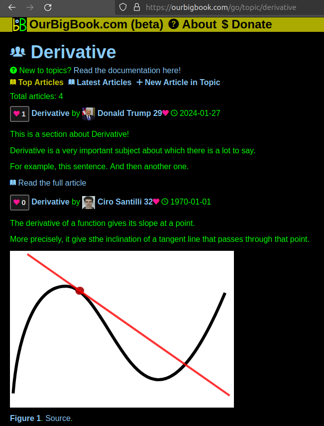
Figure 1. Screenshot of the "Derivative" topic page. View it live at: ourbigbook.com/go/topic/derivativeVideo 2. OurBigBook Web topics demo. Source. - local editing: you can store all your personal knowledge base content locally in a plaintext markup format that can be edited locally and published either:This way you can be sure that even if OurBigBook.com were to go down one day (which we have no plans to do as it is quite cheap to host!), your content will still be perfectly readable as a static site.
- to OurBigBook.com to get awesome multi-user features like topics and likes
- as HTML files to a static website, which you can host yourself for free on many external providers like GitHub Pages, and remain in full control
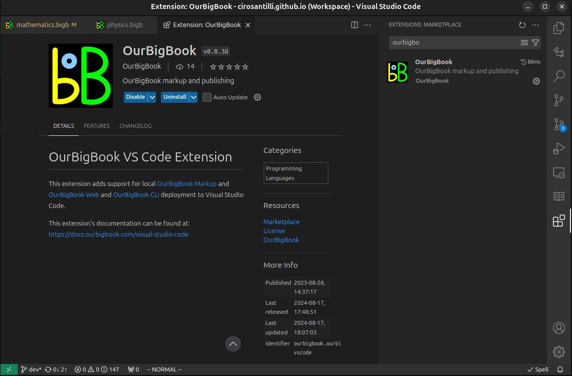
Figure 3. Visual Studio Code extension installation.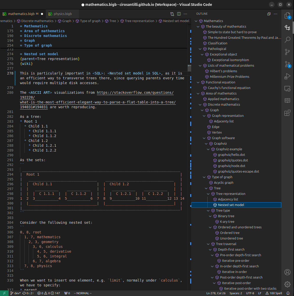
Figure 4. Visual Studio Code extension tree navigation.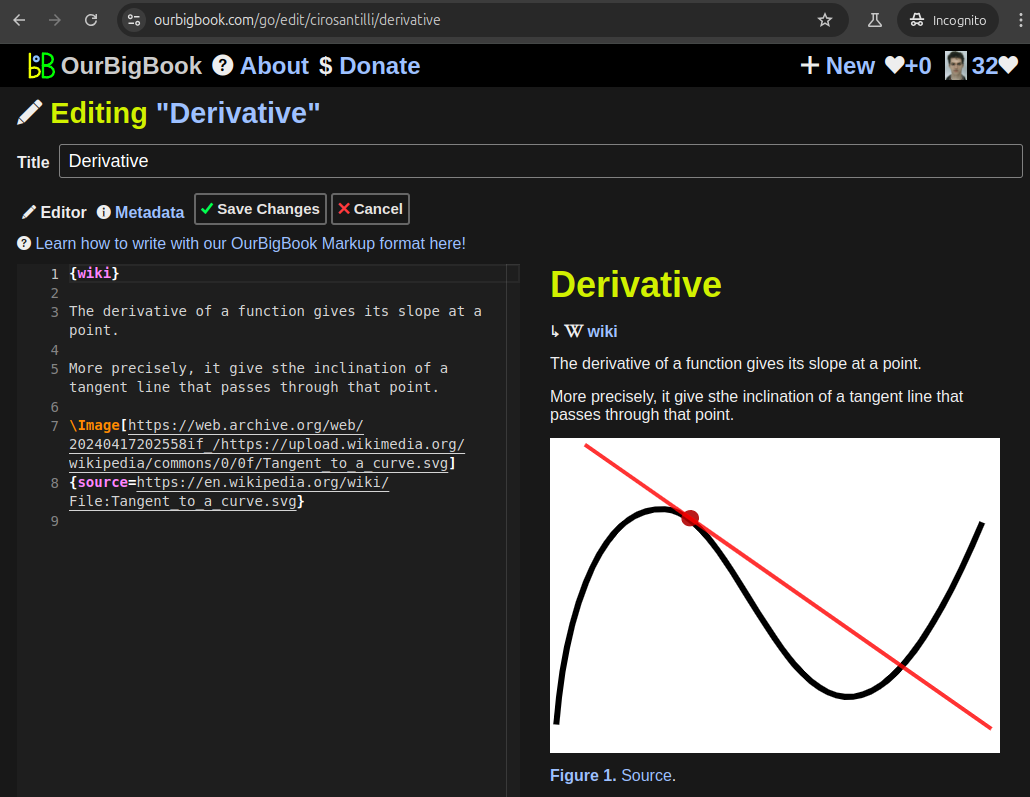
Figure 5. Web editor. You can also edit articles on the Web editor without installing anything locally.Video 3. Edit locally and publish demo. Source. This shows editing OurBigBook Markup and publishing it using the Visual Studio Code extension.Video 4. OurBigBook Visual Studio Code extension editing and navigation demo. Source. 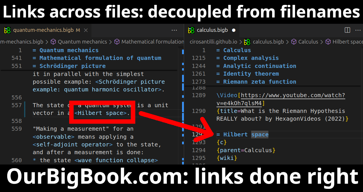
- Infinitely deep tables of contents:

All our software is open source and hosted at: github.com/ourbigbook/ourbigbook
Further documentation can be found at: docs.ourbigbook.com
Feel free to reach our to us for any help or suggestions: docs.ourbigbook.com/#contact