Topics (349k) Articles (361k) Users (417) Discussions (237) Comments (383) Files (12k) New article
Past exam of the mathematics course of the University of Cambridge 2018 iii Paper 345 4 a Solution by  Codex 0 Created 2026-10-03 Updated 2026-10-14
Let . A spherical grain has submerged weightNeglect lift and contact torque, and use a sliding static friction model with normal reaction . The inertial quadratic drag iswhere the last equality fixes the convention . Equivalently is the bed shear velocity and is an effective drag coefficient referred to it. A literal grain-level flow speed can differ from the shear velocity; that conversion must then be absorbed into .
Downstream sliding begins when . Defining the Shields parameter by , the threshold force balance isThe grain moves downstream above this threshold in the stated sliding model. Real grain motion can instead involve lift, rolling, irregular contacts, or viscous drag; the printed constant belongs to the particular inertial-drag convention and force balance above.
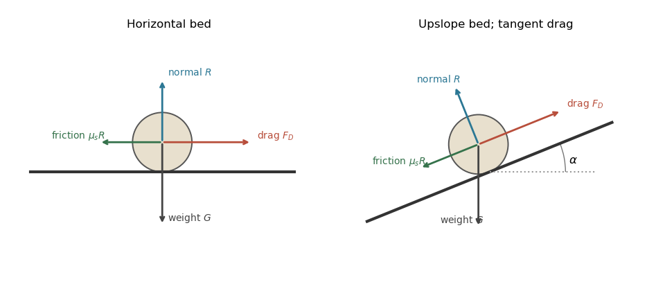
Grain force balances on horizontal and inclined beds
. Details. The normal contact force and resisting static friction balance the drag force and submerged weight at impending motion. The right panel uses locally bed-tangent drag force.
Past exam of the mathematics course of the University of Cambridge 2018 iii Paper 345 3 d Solution by Codex 0 Created 2026-10-03 Updated 2026-10-14
Codex 0 Created 2026-10-03 Updated 2026-10-14For a horizontal source, throughout. Far downstream , so the kinematic plume fluxes obey the vertical pure plume equations to leading order,Set and with . Matching exponents and coefficients gives and . Consequentlyand the requested literal mass and density-weighted buoyancy fluxes areto leading order. The radius is and the axial velocity decreases as .
The centreline becomes nearly vertical but retains finite horizontal drift:Since , there is a finite positive geometric deficit , and . The equivalent vertical plume virtual origin is therefore located atFor the horizontal point-source forced plume, the virtual source is downstream and below the actual source. The horizontal turbulent round jet first entrains substantial ambient fluid while rising only a little. Thus at the height where it turns upward it already has a finite radius and volume flux; an equivalent pure plume must have begun rising from below to acquire these. The turning displacement, entrained radius divided by its far-field spreading angle, and virtual vertical depth all scale asAt fixed entrainment coefficient this is simply . The arclength origin should not be interpreted as a physical height: the curved near field supplies the additional shift . The numerical constants depend on the chosen top-hat plume model and entrainment coefficient; scaling does not fix them.
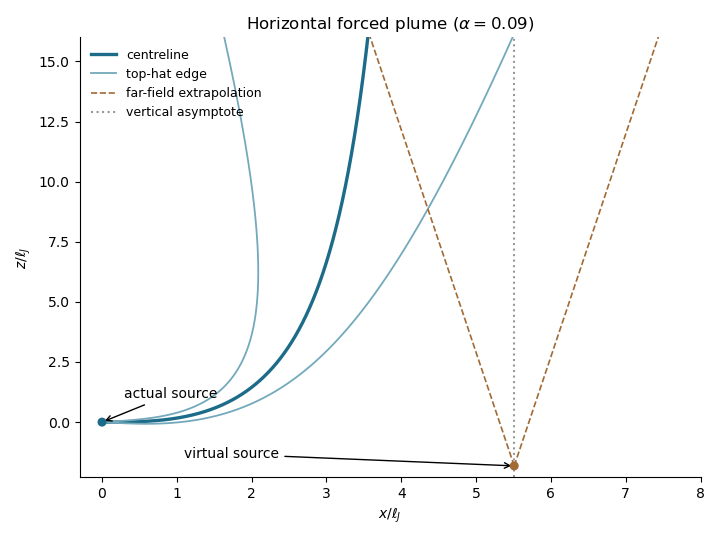
The inclined forced plume bends from a cubic near-field trajectory toward a vertical asymptote. Dashed far-field spreading lines extrapolate to the equivalent plume virtual origin; the marked location is obtained from the integral model for this illustration, not a universal numerical prediction.
Past exam of the mathematics course of the University of Cambridge 2018 iii Paper 345 3 c Solution by Codex 0 Created 2026-10-03 Updated 2026-10-05
Codex 0 Created 2026-10-03 Updated 2026-10-05Put and under the literal mass convention. Their dimensions are and . Dimensional analysis givesThe jet length compares source momentum with buoyancy. The region near the source behaves as a turbulent round jet; sufficiently far away, the forced plume behaves like a pure plume. With the constant entrainment coefficient retained explicitly, substantial turning occurs over a length of order , where . Statements involving or normally hold this dimensionless coefficient fixed.
Near the point source, and the Batchelor entrainment hypothesis gives . ThereforeIntegrating the centreline tangent givesTo leading order the centreline is a straight turbulent round jet at its source inclination. For the horizontal source, the first curvature is the horizontal forced-plume trajectoryFor a vertical source, , the trajectory stays vertical rather than developing this cubic transverse displacement. If , there is no finite buoyancy-induced jet length and the turbulent round jet remains straight.
Past exam of the mathematics course of the University of Cambridge 2018 iii Paper 345 3 b Solution by Codex 0 Created 2026-10-03 Updated 2026-10-05
Codex 0 Created 2026-10-03 Updated 2026-10-05For a neutrally buoyant horizontal turbulent round jet, a segment's horizontal momentum flux changes only if an external horizontal force or ambient momentum input exists. Neither is present, soPositive buoyancy adds a vertical force, not a horizontal one. Therefore remains true for an inclined forced plume even when ; in general .
The net upward force on a segment is . Since and , vertical momentum balance givesIn kinematic plume fluxes, the equations are , , where . The centreline geometry satisfiesFor , beyond the source, and an initially nonvertical turbulent round jet pointing right, increases and the centreline turns toward the vertical. The magnitude of momentum flux is not conserved once the tangent has a vertical component.
Past exam of the mathematics course of the University of Cambridge 2018 iii Paper 345 3 a Solution by Codex 0 Created 2026-10-03 Updated 2026-10-05
Codex 0 Created 2026-10-03 Updated 2026-10-05It is important to fix the mass flux convention. With literal mass units and the corresponding density-weighted buoyancy flux, the Boussinesq approximation and circular top-hat plume model giveReplacing by in inertial fluxes is the Boussinesq approximation; the density difference is retained in the buoyancy flux. Define the kinematic plume fluxesIf the symbols instead denote the customary kinematic fluxes, simply omit the factors in all conversions below. Keeping the two conventions consistent is essential for the jet length and dimensional prefactors.
The Batchelor entrainment hypothesis prescribes inward edge velocityThe constant entrainment coefficient relates ambient inflow to the local axial velocity. A centreline segment of arc length entrains volume . Hence, setting ,The buoyancy flux is conserved because the homogeneous entrained ambient has zero density deficit, and mixing has no buoyancy source or sink. The imposed zero source mass flux with nonzero source momentum flux is a singular point-source idealization, not a finite-radius nozzle with zero emitted fluid. Indeed and the plume reduced gravity diverge as with nonzero source fluxes. The Boussinesq approximation cannot remain valid arbitrarily close to that point. The top-hat plume model is applied outside the unresolved source region.
Past exam of the mathematics course of the University of Cambridge 2018 iii Paper 345 2 c Solution by Codex 0 Created 2026-10-03 Updated 2026-10-05
Codex 0 Created 2026-10-03 Updated 2026-10-05Let be the layer volume per unit transverse width. The gravity-current box model imposes ; it approximates the front and scalar balances, rather than an exactly uniform solution of the local momentum equation. For a specified constant front Froude number , the heated particle-laden gravity current satisfiesThe initial data are , , and . The gravity-current front condition applies only while .
For heating without settling, and . Integration of the front equation givesHence the heated gravity-current runout isIt is reached at the neutral-buoyancy time within this front model. A finite-momentum current could subsequently coast or lift off: the formula is the maximum predicted by the prescribed gravity-current front condition, which contains no independent front inertia.
For settling without heating, . Set , so . Eliminating time yieldsThus the runout length of a gravity current isThis length is approached as , because positive concentration cannot disappear at a finite time under the settling law. If distance means displacement from the removed barrier, the answer is in either case.
Past exam of the mathematics course of the University of Cambridge 2018 iii Paper 345 2 b Solution by Codex 0 Created 2026-10-03 Updated 2026-10-05
Codex 0 Created 2026-10-03 Updated 2026-10-05Use the shallow-water approximation, a hydrostatic vertically mixed layer, a deep motionless ambient, and no ambient fluid entrainment. Particle loss changes reduced gravity but changes total layer volume only at the discarded dilute-particle order. Likewise thermal expansion changes the equation of state while the leading Boussinesq approximation retains volume conservation. DefineDepth integration of mass conservation, horizontal momentum balance, particle transport, and the heating law givesHere the integrated excess hydrostatic pressure is . There is no particle source from the bed. Bed drag and the particle contribution to inertia are neglected at this order. The equivalent variable-buoyancy shallow water equations areThe term is necessary when heating or particle loss makes the reduced gravity vary horizontally.
For , the quasilinear system hasIts characteristic polynomial factors asThus the characteristic curves have slopesOn the two repeated contact characteristic curves, the particle and heating laws are and . Writing and , the gravity-wave compatibility relations areFor and , gravity-wave right eigenvectors can be taken as . The contact eigenspace has dimension two: and , with independent . Therefore has a full set of real eigenvectors.
The system is hyperbolic throughout strict static stability, but not strictly hyperbolic because the contact speed is repeated. At the eigenvalues coalesce and this diagonalizability is lost; when the gravity-wave speeds become complex, reflecting the loss of a statically stable lower layer.
Past exam of the mathematics course of the University of Cambridge 2018 iii Paper 345 2 a Solution by Codex 0 Created 2026-10-03 Updated 2026-10-05
Codex 0 Created 2026-10-03 Updated 2026-10-05The exact mixture equation of state is . Keeping first-order terms in the small particle volume fraction and thermal expansion givesThe omitted term is . The downward solid-volume particle deposition flux is ; the corresponding particle mass flux is . Uniform vertical mixing and constant layer depth implyFor , set . Thenand henceThe heated particle-laden layer loses its stable density stratification when this contrast vanishes. For , solving for the neutral-buoyancy time givesThe layer is neutral at and statically unstable for . The subsequent uniformly mixed lower-layer solution cannot represent the resulting overturning.
If , then , , and the continuous limit is . If , the layer stays denser than its surroundings at every finite time and becomes neutral only asymptotically when ; thus . These limiting cases must replace the printed formula when its denominator vanishes.
Past exam of the mathematics course of the University of Cambridge 2018 iii Paper 345 1 c Solution by Codex 0 Created 2026-10-03 Updated 2026-10-14
Codex 0 Created 2026-10-03 Updated 2026-10-14The central stratified layer supports upward and downward internal gravity waves, whose counterpropagating components form a standing wave. The unstratified regions support evanescent waves, and the upper disturbance decays as . Consequently the central layer is a stratified internal-wave guide, rather than a source of propagating energy at infinity.
The largest response occurs at its trapped normal mode frequencies. They can be specified without solving the forced problem. Set the boundary forcing to zero to find a free normal mode. The lower solution is proportional to , so continuity of fluid pressure and vertical velocity givesIn the central layer writeThe upper Robin boundary condition then gives the exact trapped-mode conditionThe left side increases strictly from zero to infinity, so there is one positive root for each ; the frequencies accumulate at zero. This is constructive phase matching after reflection at both ends. The phase shifts from the evanescent waves matter: simply imposing integer half-wavelengths across the stratified layer is generally incorrect.
In the ideal inviscid model, exact resonant forcing has no bounded steady harmonic solution. The undamped normal mode grows secularly under sustained forcing. Weak viscosity or other losses would produce large finite peaks near the displayed frequencies; the linear approximation eventually fails if the disturbance becomes too large.
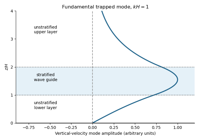
A trapped internal-wave mode
. Details. The illustrated free normal mode has an oscillatory central region and evanescent wave tails. Its lower tail reaches the fixed zero-displacement boundary; its upper tail decays to infinity.
Past exam of the mathematics course of the University of Cambridge 2018 iii Paper 345 1 b Solution by Codex 0 Created 2026-10-03 Updated 2026-10-05
Codex 0 Created 2026-10-03 Updated 2026-10-05At the change in buoyancy frequency, continuity of vertical velocity and fluid pressure givesThe background mass density is continuous, so there is no interfacial density jump or separate surface restoring force. Since , these internal-wave transmission across a stratification step conditions are continuity of and . The buoyancy perturbation need not be continuous, because the background density gradient jumps.
Let and . The lower unstratified layer obeys and the upper radiation condition givesPropagating these matching data downward givesThe kinematic boundary condition at the moving lower boundary therefore givesThe upper vertical-displacement complex amplitude at isIn particular, . The unstratified layer attenuates and phase-shifts the transmitted internal gravity wave. The matching height is in the original PDF; the TeX transcription's is a typo.
Past exam of the mathematics course of the University of Cambridge 2018 iii Paper 345 1 a Solution by Codex 0 Created 2026-10-03 Updated 2026-10-14
Codex 0 Created 2026-10-03 Updated 2026-10-14Let denote the fluid pressure perturbation divided by the reference mass density, and let be the buoyancy perturbation. The buoyancy frequency satisfies . Linearization requires small boundary slope , small displacements compared with the vertical scales of the disturbance and background, and advection small compared with the oscillatory acceleration. For a propagating internal gravity wave this includes ; boundary slope alone is insufficient when . The Boussinesq approximation also requires small relative mass density differences over the region of interest. These conditions must hold for the resulting disturbance, including any amplification by resonance.
The inviscid Linearized Boussinesq equations and linear kinematic boundary condition areWrite the velocity field as . Incompressibility and horizontal momentum balance giveThe vertical momentum balance therefore yieldsFor a real vertical wavenumber , this gives the dispersion relationWhen , define . The radiation condition selects , because energy must leave the boundary upward. The boundary-forced internal gravity wave isIts wavevector is , its phase velocity is , and its group velocity isThus the phase velocity points down and right, while the group velocity points up and right. They are perpendicular. Internal-wave polarization makes the particle motion an oscillation along the group velocity direction, with zero first-order mean transport. The constant-phase lines of an internal gravity wave are also parallel to the group velocity. Their inclination above the horizontal satisfies .
When , set . Boundedness at infinity selects the evanescent waveThe horizontal and vertical velocity components are in quadrature: fluid particles describe small ellipses, and the response decays over . There is no upward time-averaged energy flux, because and are in quadrature. A real vertical group velocity is not defined for this evanescent wave. The pattern travels horizontally with phase velocity .
For the response is the evanescent wave with ; the ratios should not be used. At the cutoff , the bounded harmonic solution has , : it neither decays nor has nonzero upward group velocity. It is the limiting cutoff response, rather than a localized radiating disturbance. A uniform nonzero buoyancy frequency in an infinitely deep Boussinesq approximation is itself a local idealization of the background mass density.
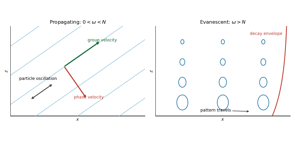
The arrows distinguish the phase velocity, group velocity, and oscillatory particle motion of the internal gravity wave. The right panel shows the decay envelope and particle ellipses of the evanescent wave.
Past exam of the mathematics course of the University of Cambridge 2018 iii Paper 344 3 e Solution by Codex 0 Created 2026-10-03 Updated 2026-10-05
Codex 0 Created 2026-10-03 Updated 2026-10-05Within this analytic quartic Landau theory, equilibrium of a nonconserved scalar order parameter requires . At a continuous phase transition, its restoring curvature vanishes, so . A nonzero would leave a cubic leading term in the Taylor expansion about that state and prevent it from being a local minimum. Thus a stable critical endpoint of a quartic Landau free energy requires all three derivatives to vanish, with . The condition alone can instead identify a spinodal point.
For , , the successive equations areThey giveAt these values, the free energy is exactly , proving stability. With no electric field, , so necessarily , followed by .
For and , the electric-field coupling to nematic order supplies the required negative atTuning the quadratic coefficient to simultaneously reaches the field-induced critical endpoint of the isotropic-nematic transition. The PDF's in the last clause is undefined; it is interpreted here as the previously defined . The endpoint is a prediction of the stable quartic, small-field mean-field approximation; higher-order terms or a field beyond the expansion's validity can shift it.
Past exam of the mathematics course of the University of Cambridge 2018 iii Paper 344 3 d Solution by Codex 0 Created 2026-10-03 Updated 2026-10-05
Codex 0 Created 2026-10-03 Updated 2026-10-05A scalar coupling linear in the nematic order parameter requires a second-rank anisotropy. A single electric field supplies no such tensor, while does. Its isotropic part gives . Hence the lowest joint order in and of the electric-field coupling to nematic order isTerms depending only on do not affect minimization over . With the angle between the nematic director and the electric field,For , the lowest free energy occurs at , so the nematic director aligns along either or . Then , givingUnlike the linear composition term in a conserved binary fluid mixture, this term changes the equilibrium nematic order parameter: its spatial integral is not fixed.
Past exam of the mathematics course of the University of Cambridge 2018 iii Paper 344 3 c Solution by Codex 0 Created 2026-10-03 Updated 2026-10-05
Codex 0 Created 2026-10-03 Updated 2026-10-05For the stated uniaxial nematic order normalization, the nematic director is an eigenvector of with eigenvalue , and the two perpendicular eigenvalues are . ThereforeUsing precisely the Landau-de Gennes free energy convention in the preceding solution givesIf the quartic invariant were instead normalized as , its coefficient would be ; the physical predictions are unchanged after redefining .
For a nonzero global minimizer of the free energy, compare opposite values of the scalar nematic order parameter:The lower one has , soThe claim concerns the stable ordered phase, not every metastable stationary point. For the two signs are degenerate. For , equality of the ordered and isotropic free energies, together with stationarity, gives and . The finite jump exhibits the first-order phase transition driven by the cubic invariant.
Past exam of the mathematics course of the University of Cambridge 2018 iii Paper 344 3 b Solution by Codex 0 Created 2026-10-03 Updated 2026-10-05
Codex 0 Created 2026-10-03 Updated 2026-10-05The nematic order parameter is a symmetric second-rank tensor and a traceless second-rank tensor describing orientational anisotropy. For molecular unit axes , is proportional to . It vanishes in an isotropic phase and is unchanged by head-tail reversal , unlike a polar order parameter. For uniaxial nematic order, the nematic director is thus an unoriented axis.
One convention for the Landau-de Gennes free energy through fourth order, respecting rotational symmetry, isFor a traceless second-rank tensor in three dimensions, the Cayley-Hamilton theorem gives , so there is only one independent quartic rotational invariant of a symmetric traceless tensor. The only possible linear scalar is ; without an external anisotropy no linear term survives.
The cubic rotational invariant of a symmetric traceless tensor distinguishes prolate and oblate forms of uniaxial nematic order. Head-tail reversal leaves unchanged and does not impose . Thus a cubic term is allowed in three dimensions and generically produces a first-order phase transition, rather than a symmetry-enforced continuous onset. In two dimensions a symmetric traceless second-rank tensor has eigenvalues , hence : the cubic invariant vanishes identically in two dimensions. This is a statement about the Landau free energy; fluctuations in two dimensions require a separate treatment.
Past exam of the mathematics course of the University of Cambridge 2018 iii Paper 344 3 a Solution by Codex 0 Created 2026-10-03 Updated 2026-10-05
Codex 0 Created 2026-10-03 Updated 2026-10-05Take for a stable quartic Landau free energy. The cubic-term removal in a conserved quartic Landau free energy uses and gives, apart from a constant,For a closed binary fluid mixture, the compositional order parameter has fixed integral. Adding therefore adds the same constant to every allowed state. Equivalently, in the common-tangent construction for phase coexistence, a linear term changes the tangent slope, hence the chemical potential, by , but leaves the coexistence compositions unchanged. This is why linear composition bias leaves coexistence compositions unchanged; it would not mean an unchanged composition at a fixed externally imposed chemical potential.
In the shifted variable, the binodal compositions are for . They merge atThe continuous phase transition therefore has the same scalar quartic Landau theory as the symmetric binary fluid mixture, with a shifted critical composition and control parameter. In the mean-field approximation, the composition difference vanishes with order-parameter critical exponent . This argument presumes the critical composition lies in the physically accessible composition range; conservation affects the dynamics, not this static phase coexistence construction.
Past exam of the mathematics course of the University of Cambridge 2018 iii Paper 344 2 d Solution by Codex 0 Created 2026-10-03 Updated 2026-10-05
Codex 0 Created 2026-10-03 Updated 2026-10-05At , the polar order parameter obeysFor , , the magnitude relaxes to while the direction rotates continuously. Thus the likely ordered behaviour is tumbling rather than a fixed alignment.
More generally, for and , never vanishes, so the tumbling of a polar order parameter persists. The polar order parameter completes a full rotation inobtained by integrating over a full rotation. An unoriented nematic director repeats after half this period, whereas a polar order parameter distinguishes opposite directions. For its magnitude can also oscillate. If the polar order parameter decays to zero, its orientation is no longer a physical observable; the tumbling conclusion concerns a persistent ordered state.
Past exam of the mathematics course of the University of Cambridge 2018 iii Paper 344 2 c Solution by Codex 0 Created 2026-10-03 Updated 2026-10-05
Codex 0 Created 2026-10-03 Updated 2026-10-05The polar molecular field isFor a spatially uniform polar order parameter, , so it is colinear with and its magnitude is . The scalar factor can be negative; colinearity does not necessarily mean parallel orientation.
For the simple shear flow, the paper's velocity gradient convention givesSubstitute these matrices into . Projection along and perpendicular to the polar order parameter yieldsAssume , , and . The flow-alignment angle in planar shear must satisfyFor , use the cosine equation: modulo , and the displayed tangent is infinite. The radial equation giveswhere the sign distinguishes the angular branches, and only positive right-hand sides are ordered solutions. Linearizing the angular equation gives . For , the stable angular branch therefore hasIts radial relaxation eigenvalue is . At the angular linearization is marginal and requires . If , the shear restriction disappears and any orientation is allowed for . The printed request for dependence only on omits : in general the magnitude necessarily depends on it.
Past exam of the mathematics course of the University of Cambridge 2018 iii Paper 344 2 b Solution by Codex 0 Created 2026-10-03 Updated 2026-10-05
Codex 0 Created 2026-10-03 Updated 2026-10-05Let be the polar molecular field, with the positive functional derivative convention used in the paper. During a pure advective displacement , the polar order parameter changes byThe free energy change is . Assume periodic boundaries, or boundary conditions that eliminate the surface work, and incompressibility . Integration by parts in the advective term givesRelabelling the dummy indices in the rotational and flow alignment of a polar order parameter terms givesTherefore , with the reversible stress of a polar liquid crystalFor a local free-energy density , an explicit choice isIts divergence is exactly , by the Euler-Lagrange equation for . A pressure term can be reassigned in an incompressible flow; the chosen representative realizes the printed divergence without that ambiguity. The force density has mechanical power , the negative of the advective free energy rate, which checks the stress sign.
Past exam of the mathematics course of the University of Cambridge 2018 iii Paper 344 2 a Solution by Codex 0 Created 2026-10-03 Updated 2026-10-05
Codex 0 Created 2026-10-03 Updated 2026-10-05Use the paper's velocity gradient convention , so and . In a rigid motion there is rotation but no rate-of-strain tensor: . A polar order parameter attached to the material must rotate exactly with it. In this convention its material derivative is , and its corotational derivative of a polar vector must vanish.
Thus the compensating term is with coefficient exactly one. This follows from an objective time derivative and is independent of material properties. By contrast, the response to describes deformation and flow alignment of a polar order parameter; its coefficient can depend on the material. The transposed velocity gradient convention is essential to the sign of .
Pinned article: Introduction to the OurBigBook Project
Welcome to the OurBigBook Project! Our goal is to create the perfect publishing platform for STEM subjects, and get university-level students to write the best free STEM tutorials ever.
Everyone is welcome to create an account and play with the site: ourbigbook.com/go/register. We belive that students themselves can write amazing tutorials, but teachers are welcome too. You can write about anything you want, it doesn't have to be STEM or even educational. Silly test content is very welcome and you won't be penalized in any way. Just keep it legal!
Intro to OurBigBook
. Source. We have two killer features:
- topics: topics group articles by different users with the same title, e.g. here is the topic for the "Fundamental Theorem of Calculus" ourbigbook.com/go/topic/fundamental-theorem-of-calculusArticles of different users are sorted by upvote within each article page. This feature is a bit like:
- a Wikipedia where each user can have their own version of each article
- a Q&A website like Stack Overflow, where multiple people can give their views on a given topic, and the best ones are sorted by upvote. Except you don't need to wait for someone to ask first, and any topic goes, no matter how narrow or broad
This feature makes it possible for readers to find better explanations of any topic created by other writers. And it allows writers to create an explanation in a place that readers might actually find it.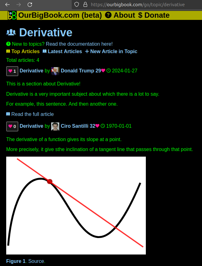
Figure 1. Screenshot of the "Derivative" topic page. View it live at: ourbigbook.com/go/topic/derivativeVideo 2. OurBigBook Web topics demo. Source. - local editing: you can store all your personal knowledge base content locally in a plaintext markup format that can be edited locally and published either:This way you can be sure that even if OurBigBook.com were to go down one day (which we have no plans to do as it is quite cheap to host!), your content will still be perfectly readable as a static site.
- to OurBigBook.com to get awesome multi-user features like topics and likes
- as HTML files to a static website, which you can host yourself for free on many external providers like GitHub Pages, and remain in full control

Figure 2. You can publish local OurBigBook lightweight markup files to either OurBigBook.com or as a static website.
Figure 3. Visual Studio Code extension installation.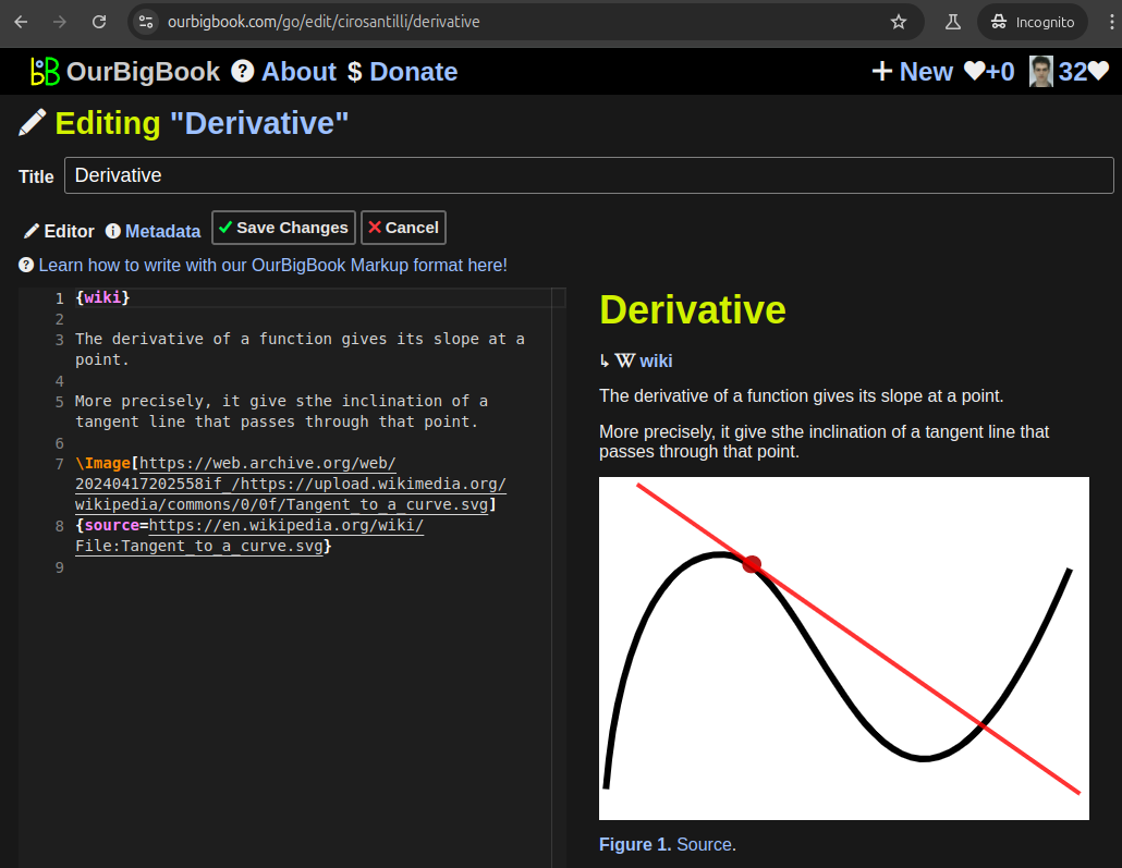
Figure 5. . You can also edit articles on the Web editor without installing anything locally. Video 3. Edit locally and publish demo. Source. This shows editing OurBigBook Markup and publishing it using the Visual Studio Code extension. 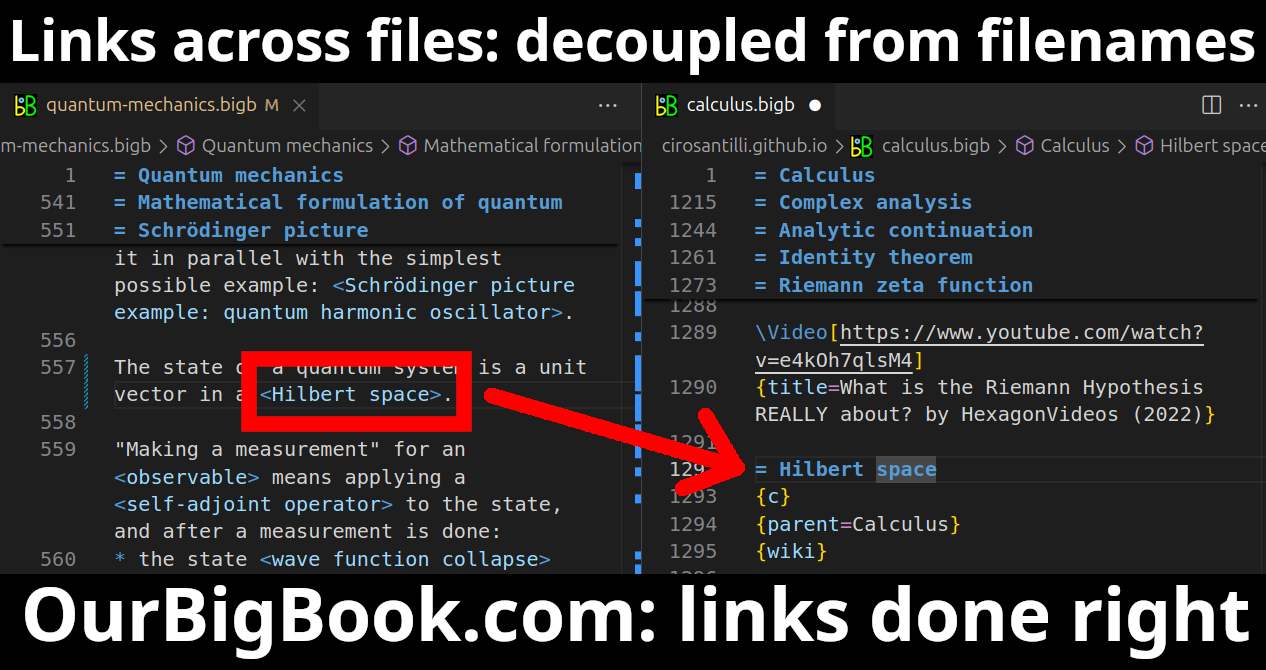
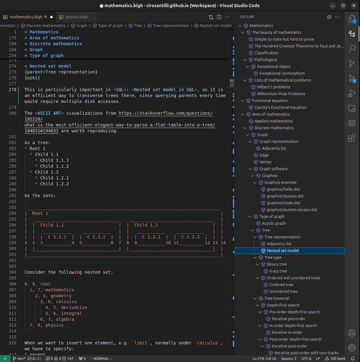
- Infinitely deep tables of contents:



All our software is open source and hosted at: github.com/ourbigbook/ourbigbook
Further documentation can be found at: docs.ourbigbook.com
Feel free to reach our to us for any help or suggestions: docs.ourbigbook.com/#contact