A metric space $(X,d)$ is a complete metric space if every Cauchy sequence in $X$ converges to a point of $X$. Explicitly, the hypothesis isand the conclusion is that some $x\in X$ satisfies $d(x_n,x)\to 0$.

It is a sequentially compact space if every sequence in $X$ has a convergent subsequence whose limit of a sequence belongs to $X$.

It is a connected space if there are no disjoint nonempty open subsets $U,V$ of $X$ with $X=U\cup V$. Here openness refers to the metric topology of $X$.

It is a path-connected space if, for every $x,y\in X$, there is a continuous map $\gamma :[0,1]\to X$ with $\gamma (0)=x$ and $\gamma (1)=y$. Such a map is a path. Every path-connected space is a connected space: a separation would pull back along a path joining its two sides to a separation of the interval $[0,1]$.

Let $n=2m\ge 2$. Between the two middle order statistics, $k=m$ and the slope $A^{\prime }(\mu )=2m-n$ is zero. To the left $A$ decreases and to the right it increases. Consequently all joint maximum-likelihood estimates arewhere the constant minimum isThe strict positivity follows from distinct observations. Thus the location maximum-likelihood estimate is not unique, while the rate maximum-likelihood estimate is unique and the same for every location in the displayed interval. Choosing the arithmetic midpoint of the two middle values is the usual sample median convention and gives one member of this entire maximizing family.

For each fixed $\lambda >0$, maximizing the likelihood function over $\mu$ is equivalent to minimizing $A(\mu )={\sum }_i|x_i-\mu |$. Order the distinct observations as $x_{(1)}<\cdots <x_{(n)}$ and write $n=2m+1$. Between successive order statistics, with exactly $k$ observations to the left,Thus $A$ decreases up to $x_{(m+1)}$ and increases after it. Its unique minimum is at the sample median:At a fixed $\mu$ with $A(\mu )>0$, the log-likelihood function has derivative $n/\lambda -A(\mu )$ and second derivative $-n/{\lambda }^2<0$, so its unique maximizing rate is $n/A(\mu )$. The maximized likelihood function is $(n/[2eA(\mu )]{)}^n$, which increases when $A(\mu )$ decreases. Hence the joint maximum-likelihood estimates areThis is Laplace location and scale maximum likelihood, expressed with the reciprocal scale.

A finite rate maximum-likelihood estimate requires a positive total absolute deviation. For distinct observations and odd $n\ge 3$, that condition holds. For $n=1$, however, $\mu =x_1$ gives $A(\mu )=0$ and $L=\lambda /2\to \infty$ as $\lambda \to \infty$. There is no finite joint maximum-likelihood estimate in the stated parameter space; the formula with zero denominator is not an admissible estimate.

The joint maximum-likelihood estimators are functions of the observations selecting a maximizing parameter pair:The estimates after observation maximize the same likelihood function with $X_i=x_i$. Maximization may be nonunique, as for an even sample size, or may fail to yield a finite admissible pair, as in the one-observation case below. The definition does not turn a boundary supremum into an attained maximum.

By independence, the likelihood function is the product of the individual probability density functions:Writing $A(\mu )={\sum }_i|x_i-\mu |$, the log-likelihood function is $\ell =n\ln \lambda -n\ln 2-\lambda A(\mu )$. Here $\lambda$ is a rate, the reciprocal of the scale in the usual Laplace distribution notation.

For this rate parametrization of the Laplace distribution, $\mu$ is its mean and median. By symmetry, $\mathbb{E}(X-\mu )=0$, while $|X-\mu |$ has exponential distribution with rate $\lambda$, soThe integral follows by two applications of integration by parts. The central limit theorem therefore givesWith known $\lambda$ and the supplied cutoff 2, an approximate 95% confidence interval isThis known-rate Laplace location confidence interval uses the sample mean; the later maximum-likelihood estimator of location need not be used to construct this valid asymptotic confidence interval.

At sample size 100, keep essentially the same numerical confidence interval, but treat its calibration as approximate. For independent heights with finite, nonzero variance, the central limit theorem makes the sample mean approximately normally distributed, and the sample variance consistently estimates the population variance. Hence the studentized sample mean is approximately standard normal even without a normal distribution for individual heights.

Using the permitted cutoff 2 givesA Student t-distribution cutoff gives a similar approximation for large sample size, but its justification at fixed sample size is no longer exact. Extreme skewness or influential outliers could make 100 observations insufficient for accurate coverage probability; abandoning normality alone supplies no specific numerical correction. The sampling with replacement assumption still precludes a finite population correction.

The independent uniform choices from the student list describe sampling with replacement. Under the stated independent normal distribution model for the heights, the population variance is unknown and the given $8.5$ cm is the sample standard deviation $s$. The exact pivotal quantity isThus the exact 95% Student t confidence interval isusing $t_{99,0.975}\approx 1.9842$. The supplied approximation $\Phi (2)=0.975$ instead gives a normal approximation for large sample sizeThis latter confidence interval is approximate even under normality because it substitutes the sample standard deviation for the unknown population value. There is no finite population correction under the specified independent selections. Interpreting the finite student list literally as a discrete population makes normality an idealized model; it does not justify changing the stated sampling design.

It is single-linkage clustering. Its intercluster distance is the smallest cross-pair Euclidean distance. Successive nearby points can join around the ring and within the dense central cloud before any edge crosses the gap between them. Equivalently, at a threshold below the between-group gap but above the lengths needed to connect each group, the single-linkage clustering components are precisely the central group and the ring.

Complete-linkage clustering uses the largest cross-pair Euclidean distance. Opposite points on the ring are far apart, so an intact ring has a large diameter. That rule favors compact pieces and can attach a ring segment to the center before all ring segments join. The visible gap and short links within each group explain why single-linkage clustering recovers the two intended clusters in cluster analysis in this example; it is not a universal guarantee for arbitrary noisy rings.

With two distinct centroids, K-means clustering assigns points on opposite sides of their nearest-centroid decision hyperplane, which in two dimensions is a straight line. This constraint explains the typical outcomes in the three source plots; exact assignments depend on initialization and the realized points.

Dataset A: one cluster in cluster analysis contains most of the horizontal cloud and the bottom of the vertical cloud; the other contains the upper part of the vertical cloud. The two visually elongated groups are poorly matched to squared Euclidean distance from their centroids. Points at the lower end of the vertical group can be closer to the horizontal group's centroid, so the two original shapes need not be recovered intact.

Dataset B: a roughly straight cut divides the ring and generally the central cloud between the two clusters in cluster analysis. A Voronoi cell for either centroid is a half-plane; it cannot select a surrounding ring while excluding its center. The cut's direction can vary because the geometry is approximately rotationally symmetric.

Dataset C: the two dense lower clouds typically receive different centroids. The much smaller upper cloud is absorbed into one or divided between both clusters in cluster analysis, according to the nearly vertical separating line. With $K=2$, the objective usually benefits more from separating the two large clouds than from spending one centroid on the sparse third group. These are typical qualitative outcomes, rather than guarantees about every initialization.

Complete-linkage clustering defines the dissimilarity between clusters in cluster analysis $A,B$ as $d_{\mathrm{CL}}(A,B)={\max }_{i\in A,j\in B}{d}_{ij}$. Remove point 6 and first merge 1 with 4 at height $0.67$. The distances from $\{1,4\}$ to 2, 3, 5 are respectivelyThe next merge therefore attaches 2 at $1.41$. Now the distances from $\{1,2,4\}$ to 3 and 5 are $2.95$ and $3.32$, whereas $d_{35}=2.82$. Merge 3 and 5 at $2.82$. The final distance between the two remaining clusters in cluster analysis is the largest cross-entry, $3.32$. Thus the dendrogram has merges

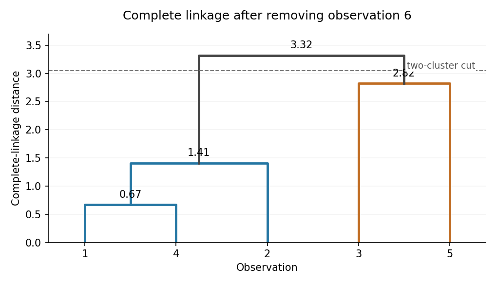
Cutting strictly between heights $2.82$ and $3.32$ gives the two clusters in cluster analysisThe figure is an original drawing of these computed merges.

Every Euclidean distance obeys the triangle inequality. The three recorded entries $d_{14}=0.67$, $d_{16}=2.88$ and $d_{46}=4.37$ violate it:At least one of $0.67,2.88,4.37$ must be incorrect. Two are in the final row as required. The gap is far larger than any possible rounding of entries to two decimal places.

Compute fitted responses ${\hat{y}}_i=\hat{\alpha }+\hat{\beta }{x}_i$ and regression residuals $e_i=y_i-{\hat{y}}_i$. A conventional residual plot shows $e_i$ against ${\hat{y}}_i$ or $x_i$; plotting against observation order additionally looks for runs. One checks for curvature, changing spread and other structure rather than random scatter around zero.

An ordinary residual plot need not reveal this failure of independence. The errors have constant mean zero, constant variance one and zero pairwise covariances, so the usual trend and changing-variance clues need not appear. A visually patternless residual plot cannot validate independence; fitted regression residuals themselves also share the fitted coefficients even when the true errors are independent.

There is detectable dependence in the magnitudes. The Gaussian fourth moment is $\mathbb{E}{\eta }_i^4=3$, giving for every adjacent pairFor $i=1$, the product is ${\eta }_1^4{\eta }_2^2$; for $i\ge 2$, it is ${\eta }_{i-1}^2{\eta }_i^4{\eta }_{i+1}^2$, with the same expected value 3. Large magnitudes tend to occur together. A lagged plot of squared regression residuals or a test directed at dependence in their squares is more informative. Thus recognition is possible with suitable diagnostics, but is not guaranteed by the standard residual plot requested here.

The least-squares estimators depend only on the observed responses and design, so the formulas in i still hold. Their variances and covariance need only the error covariance matrix, now $I_n$. ThereforeFor example the first formula follows from $\mathrm{Var}({\sum }_i{x}_i{ϵ}_i)={\sum }_i{x}_i^2$, and the second from ${\sum }_i{x}_i=0$. The formulas remain the same as before with ${\sigma }^2=1$; this calculation does not establish independence or a normal distribution for the estimators.

Independence of the centered standard normal random variables gives $\mathbb{E}{ϵ}_i=0$ for every $i$. AlsoFor nonadjacent indices, the underlying sets of $\eta$ variables are disjoint, so the errors are independent and have zero covariance. For adjacent indices with $i\ge 2$,The first adjacent pair separately gives $\mathbb{E}[{ϵ}_1{ϵ}_2]=\mathbb{E}[{\eta }_1^2{\eta }_2]=0$. HenceThese adjacent products of independent Gaussian variables are uncorrelated random variables even though adjacent errors share a factor and are dependent.

For the random vector $\mathbf{ϵ}=({ϵ}_1,\dots ,{ϵ}_n{)}^{\top }$, its covariance matrix isIts diagonal entries are variances, and its off-diagonal entries measure pairwise covariance. Finite second moments make every entry well defined.

They need not be independent. For a counterexample take $n=2$, $x_1=-1$, $x_2=1$, and independent errors taking $-1,1$ with equal probability. ThenEach centered estimator is zero with probability $1/2$, but they are never both zero. Their zero events therefore violate independence.

A sufficient additional assumption is that the errors have a common normal distribution. The two estimators are then Jointly Gaussian, being linear combinations of the independent Gaussian random variables. Their zero covariance, established in iii, implies independence of uncorrelated jointly normal variables. Normal errors are a sufficient condition here, not a claim that no other error probability distribution could ever work.

Here $\hat{\alpha }=\alpha +n^{-1}{\sum }_i{ϵ}_i$. By linearity of covariance and independence,Thus the two estimators are uncorrelated random variables.