The Euclidean norm is invariant under an orthogonal matrix, so the full singular value decomposition givesThe second term is independent of $x$; the first attains its unique minimum zero because $\Sigma$ is an invertible matrix. The linear least squares solution is thereforeHere $A^{+}=V{\Sigma }^{-1}{U}^T$ is the Moore-Penrose inverse, and the fitted vector is the orthogonal projection $A{x}_{\ast }=U{U}^{T}b$ onto the image of a linear map defined by $A$.

With the singular value decomposition supplied, forming $U^{T}b$ costs $O(mn)$ arithmetic operations, diagonal scaling costs $O(n)$, and multiplication by $V$ costs $O(n^2)$. Since $m\ge n$,One need not form $U_{\perp }$, $A^{+}$ or $A^{T}A$ to calculate $x_{\ast }$. Computing the needed thin singular value decomposition first has standard dense cost $O(m{n}^2)$; explicitly forming an entire $m\times m$ orthogonal completion can require additional work when $m$ is much larger than $n$.

For $m=n$, $U$ and $V$ are square orthogonal matrices. Multiply the linear system successively by $U^T$, ${\Sigma }^{-1}$ and $V$ to obtainWith the singular value decomposition already supplied, compute $c=U^{T}b$, divide $c_j$ by ${\sigma }_j$, then form $x=Vc$. The two dense matrix-vector products each cost $O(n^2)$ arithmetic operations in Big O notation, and the diagonal scaling costs $O(n)$. ThusIf the singular value decomposition first has to be computed, its usual dense cost is $O(n^3)$; that is a separate setup cost and can be reused for further right-hand sides.

All $n$ singular values are positive, so $\Sigma$ and $V$ are invertible matrices and $A$ has matrix rank $n$. The image of a linear map is thereforewith those columns furnishing an orthonormal basis. Also $Ax=0$ implies $\Sigma V^{T}x=0$ and hence $x=0$. ThusFinally $A^{T}z=V\Sigma U^{T}z=0$ exactly when $U^{T}z=0$. The remaining columns of the full orthogonal matrix span this orthogonal complement:If $m=n$, this last null space also equals $\{0\}$ and has the empty basis.

Set $W=\mathrm{diag}(w_0,\dots ,w_n)$. For column indices $j,k\in \{1,\dots ,n+1\}$, the product $P_{j-1}{P}_{k-1}$ has polynomial degree at most $2n$, so exactness of Gauss-Legendre quadrature and orthonormality giveThus $Q=W^{1/2}A$ is a square matrix with $Q^{T}Q=I$, and therefore is an orthogonal matrix: $Q{Q}^T=I$ as well. It follows thatEquivalently, the rows of the generalized Vandermonde matrix are orthogonal andThe normalization matters: here $P_{n+1}=\sqrt{(2n+3)/2}{L}_{n+1}$, where $L_{n+1}$ is the conventional Legendre polynomial used above. Thus a formula containing only the nodes and the question's orthonormal polynomials isThis identity is the discrete orthogonality of Gaussian quadrature.

Truncate the Chebyshev series at the full degree of precision of a quadrature rule:Since $|T_j(x)|\le 1$ on $[-1,1]$, the geometric series estimate givesThe same bound proves uniform convergence of the original Chebyshev series, so its sum and the tail estimate are justified. Gauss-Legendre quadrature is exact on $s_{2n+1}$. Its positive quadrature weights sum to $2$, henceTherefore one explicit choice proving exponential convergence of Gaussian quadrature isUsing exactness through polynomial degree $2n+1$ doubles the exponent compared with truncating at polynomial degree $n$.

Let $L_{n+1}$ denote the conventional Legendre polynomial, normalized by $L_{n+1}(1)=1$. The $n+1$ quadrature nodes are its distinct polynomial roots in $(-1,1)$. For these nodes form the Lagrange cardinal polynomialsChoose the quadrature weights by integrating these polynomials:An equivalent standard formula isThe reason for selecting these quadrature nodes is the resulting degree of precision of a quadrature rule. For any polynomial $p$ of polynomial degree at most $2n+1$, polynomial division givesThe orthogonality of the Legendre polynomial makes ${\int }_{-1}^1{L}_{n+1}s=0$, while $p(x_i)=r(x_i)$ at each quadrature node. The definition of the quadrature weights integrates $r$ exactly, soIn particular, ${\sum }_i{w}_i=2$. Applying this exactness to ${\ell }_i^2$ also proves $w_i={\int }_{-1}^1{\ell }_i(x{)}^{2}dx>0$.

Let $r=f-p_n$ be the continuous function describing the error. The preceding orthogonality equations sayIf $r$ vanishes identically, any $n+1$ distinct points work. If $r$ already has at least $n+1$ distinct zeros, the assertion also follows. Suppose instead that it has at most $n$ distinct zeros. Among its interior zeros, list those at which its sign changes as $t_1<\cdots <t_m$, where $m\le n$, and define the polynomialwith $q=1$ if $m=0$. Between consecutive zeros of $r$, its sign is constant by the intermediate value theorem. At each $t_j$, both $r$ and $q$ change sign; at every other zero of $r$, neither sign changes. Hence $rq$ has one fixed sign throughout $[-1,1]$ wherever it is nonzero. Replacing $q$ by $-q$ if necessary makes $rq\ge 0$ everywhere.

Since $r$ is not identically zero and $q$ has only finitely many zeros, $rq$ is strictly positive on some open interval. Positivity of $w$ givescontradicting orthogonality because $q\in {\mathcal{P}}_n$. ThusThis is the interpolation property of weighted least-squares polynomial approximation. It supplies interpolation nodes depending on $f$ and $w$, rather than nodes prescribed in advance.

Write ${\mathcal{P}}_n$ for the vector space of polynomials of polynomial degree at most $n$, and put $p_n(x)={\sum }_{j=0}^n{a}_j{x}^j$. As the question calls the weighted integral an inner product, its finiteness is implicit; for example, a positive integrable weight $w$ suffices for all the continuous functions involved here.

For every $q\in {\mathcal{P}}_n$, differentiating the squared weighted norm $\Vert f-p_n-tq{\Vert }_w^2$ at its minimum $t=0$ gives the orthogonality equationsIn particular, the requested linear system isIts Gram matrix $G_{kj}={\int }_{-1}^{1}w(x)x^{k+j}dx$ is a symmetric positive-definite matrix: for any nonzero vector $a$,Indeed a nonzero polynomial is nonzero on some open interval, and the weight is positive. Therefore $G$ is an invertible matrix, proving uniqueness. Conversely, if these equations hold, the Pythagorean theorem in an inner-product space gives, for every $q\in {\mathcal{P}}_n$,so the solution really is the unique best approximation.

A stable terminal product obeys ${\dot{N}}_c={\lambda }_b{N}_b$. Conservation of the number of chain members gives $N_a+N_b+N_c=N_{a0}+N_{c0}$ when $N_{b0}=0$. Therefore, for distinct nuclear decay constants,Set $N_{c0}=0$ for an initially absent terminal product. For equal nuclear decay constants,Both expressions have ${\dot{N}}_c(0)=0$ because the intermediate population initially vanishes; their leading growth is $\frac{1}{2}{N}_{a0}{\lambda }_a{\lambda }_b{t}^2$. For positive nuclear decay constants, $N_c$ increases monotonically to $N_{c0}+N_{a0}$.

For $N_{b0}=0$, differentiate the distinct-nuclear decay constant result:Equating the production and loss terms gives $e^{({\lambda }_b-{\lambda }_a)t}={\lambda }_b/{\lambda }_a$, henceFor positive nuclear decay constants and $N_{a0}>0$, this is positive regardless of their ordering. Initially ${\dot{N}}_b>0$, while $N_b\to 0$ at late times; the stationary point is the unique maximum. At that time ${\lambda }_a{N}_a={\lambda }_b{N}_b$. If the nuclear decay constants are equal, differentiating $\lambda N_{a0}t{e}^{-\lambda t}$ gives $\boxed{t_{\max }=1/\lambda }$, also the continuous limit of the expression above.

For a closed unit-branching radioactive decay chain, the rate equations areThe first gives $N_a=N_{a0}{e}^{-{\lambda }_{a}t}$. Multiply the second by its integrating factor $e^{{\lambda }_{b}t}$:Integrate from zero to $t$. For ${\lambda }_a\ne {\lambda }_b$,soThe coefficients can individually be negative; the physical population is nonnegative because the production integral is nonnegative. For equal nuclear decay constants ${\lambda }_a={\lambda }_b=\lambda$, the finite limit isA sum of two constant-coefficient copies of the same exponential function cannot represent this limit; the $t$ factor is essential.

This is the charge-and-parity-conjugate reaction of part (i). There are $t$-channel Z boson and crossed W boson contributions, with all fermion arrows reversed relative to part (i). For matched unpolarized kinematics and negligible CP violation,Combining all four results in the regime specified in part (i),In particular, conjugating both initial particles restores the part-(i) rate; conjugating the neutrino alone does not. Initial spin polarization and energies near a weak-boson mass require a separate comparison.

Both $t$-channel Z boson exchange and $s$-channel annihilation $e^{-}{\bar{\nu }}_e\to W^{-\ast }\to e^{-}{\bar{\nu }}_e$ occur. Replacing the incident neutrino by an antineutrino interchanges the two chiral angular weights. In the same contact-interaction regime,At $x=0.231$ the factor is $0.2315$, between parts (i) and (ii). The comparison is energy dependent outside this regime: near $s=m_W^2$, the annihilation channel has a W boson resonance, and the low-energy formula is inapplicable.

Only $t$-channel Z boson exchange contributes at leading order. A W boson would connect ${\nu }_{\mu }$ to ${\mu }^{-}$, rather than to $e^{-}$, and therefore does not supply this elastic channel. With the assumptions and normalization of part (i),For the illustrative value $x=0.231$, the dimensionless factors in parts (i) and (ii) are $0.5521$ and $0.09015$. The electron-flavor reaction is therefore about $6.1$ times as large in this limit. This uses the weak flavour selection in neutrino-electron scattering, not a hypothetical flavor-changing neutral vertex.

There is a $t$-channel Z boson contribution and a crossed, $u$-channel W boson contribution. The latter pairs the incoming electron neutrino with the outgoing electron, and the incoming electron with the outgoing electron neutrino. Both contribute coherently to the same elastic final state.

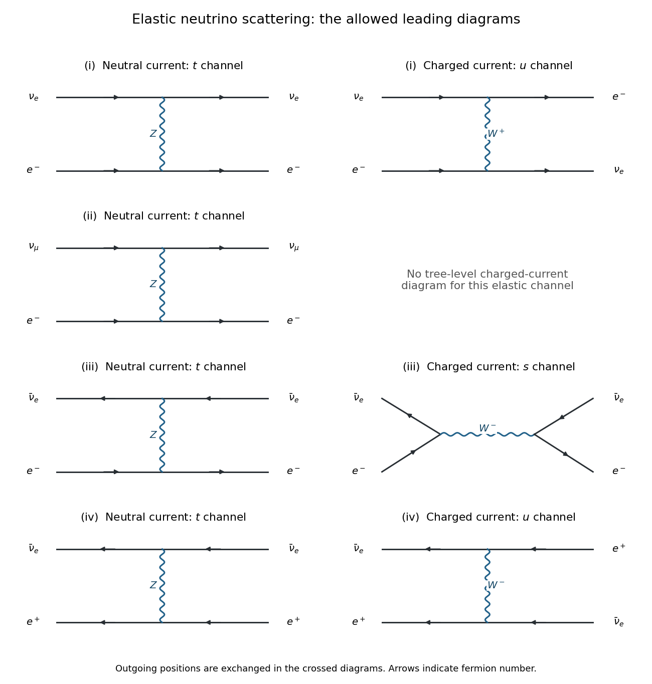
For a concrete comparison, take unpolarized targets, the same Mandelstam invariant $s$ in all four reactions, and $m_e^2\ll s\ll m_W^2$. In a stationary-electron experiment this includes $E_{\nu }\gg m_e$ with $s\simeq 2m_e{E}_{\nu }$. Define $x={\sin }^2{\theta }_W$, using the weak mixing angle, and ${\sigma }_{\ast }=G_F^{2}s/\pi$. The weak neutral current has chiral couplings $g_L=x-1/2$, $g_R=x$; the weak charged current shifts $g_L$ by one. ConsequentlyThe factor $1/3$ comes from integrating the opposite-chirality angular weight: in the massless limit ${\int }_0^1(1-y{)}^{2}dy=1/3$. Thus the relative rate depends on the chiral couplings and their interference, rather than simply on the number of diagrams.

The set $I^n$ consists precisely of points whose first $n$ positions $x,f(x),\dots ,f^{n-1}(x)$ all lie in $L\cup R$. HenceDeleting the first position preserves this condition, proving $f(\Lambda )\subseteq \Lambda$. For the reverse inclusion, if $y\in \Lambda$, take $x=g_L(y)$. Then $x\in L$ and $f^k(x)=f^{k-1}(y)\in L\cup R$ for every $k\ge 1$. Thus $x\in \Lambda$ and $f(x)=y$. In fact both inverse branches give preimages in $\Lambda$. Thereforewhich proves full invariance, not merely forward invariance.

For any infinite symbolic sequence $s$, the itinerary cylinders $I_{s_1\cdots s_n}$ are nonempty compact nested intervals. The nested interval theorem gives at least one point in their intersection. Every $x\in \Lambda$ has a unique itinerary because $L\cap R=\varnothing$. To justify that the itinerary also determines a unique point, it suffices to show the interval lengths shrink. The fact that logistic inverse branches contract in an angular coordinate works for every $\mu >4$; a direct claim that $|g_L^{\prime }|,|g_R^{\prime }|<1$ in the original coordinate would fail for some $\mu$ just above four.

Use the homeomorphism $h(u)={\sin }^2(\pi u/2)$ of $[0,1]$. The transformed inverse branches areTheir derivatives satisfyThe inequality follows by squaring and using $4/\mu <1$. Thus every length-$n$ transformed itinerary cylinder has length at most ${\mu }^{-n/2}$. Since $|h^{\prime }|\le \pi /2$, its original interval has length at most $(\pi /2){\mu }^{-n/2}$ and shrinks to a point. This gives the claimed one-to-one identification with the one-sided full shift.

Finally part (ii) givesThus $f$ acts by the left shift. The identification is a topological conjugacy: matching long prefixes forces closeness by the shrinking estimate, while distinct finite itinerary cylinders are disjoint compact sets and so their inverse coding is continuous. In particular $f$ need not be one-to-one on $\Lambda$, just as a one-sided left shift has two possible first symbols before any given tail.

Write $G=g_{s_1}\circ \cdots \circ g_{s_{n-1}}$. Because $g_{s_n}([0,1])\subseteq [0,1]$, taking the image under the same function composition givesThis uses preservation of set inclusion by every function, so decreasing inverse branches cause no difficulty. Since $f\circ g_L=f\circ g_R={\mathrm{id}}_{[0,1]}$, cancellation of the first inverse branch gives the equality of imagesThese compact intervals are itinerary cylinders: their symbols record successive positions under iteration of a map. In particular,Conversely these three memberships allow successive substitution of the appropriate inverse branches, and therefore characterize $I_{LLR}$ exactly.

Solving $\mu x(1-x)=1$ by the quadratic formula givesFor $\mu >4$, $0<x_{-}<1/2<x_{+}<1$. On $L=[0,x_{-}]$ the derivative $f^{\prime }(x)=\mu (1-2x)$ is strictly positive, while on $R=[x_{+},1]$ it is strictly negative. Thus the restrictions are strictly monotonic functions. Their endpoint values areBy continuity and strict monotonicity, each restriction maps its interval bijectively onto $[0,1]$, with opposite orientations. The corresponding inverse functions are

Construct one infinite binary sequence $u$ by concatenating every binary word of length one, then every word of length two, then every word of length three, and so on, in lexicographic order within each length. Every finite binary word occurs somewhere in $u$.

Given any target sequence $s$ and any $\eta >0$, choose $N$ such that $2^{-N}<\eta$. The word $s_1\cdots s_N$ occurs in $u$, beginning after some $k$ symbols. Thus ${\sigma }^{k}u$ agrees with $s$ in its first $N$ positions, and the prescribed metric givesEvery open open ball about every point therefore meets the forward orbit of $u$. This forward orbit is dense in $\Sigma$. The argument identifies finite-prefix cylinder sets as arbitrarily small neighborhoods in this metric; no binary-expansion convention for real numbers is needed.

The space $\Sigma$ of all infinite binary sequences is uncountable by the Cantor diagonal argument: given any list $s^{(1)},s^{(2)},\dots$, the sequence $t_i=1-s_i^{(i)}$ differs from its $i$th entry at position $i$, so it is absent from the list. Part (i) shows that only countably many sequences are periodic. Their complement is therefore uncountable.

Each forward orbit $\{{\sigma }^n(s):n\ge 0\}$ is countable. If there were only countably many nonperiodic forward orbits, their union together with the periodic points would be countable, contradicting the preceding argument. Hence there are uncountably many nonperiodic orbits, rather than merely uncountably many nonperiodic starting points.

One can also exclude eventual periodicity. An eventually periodic sequence is specified by a finite initial word and a finite repeating word, so only countably many exist. Removing all of them still leaves an uncountable set. This proves the assertion even if “nonperiodic” is understood to exclude orbits that eventually enter a periodic orbit.