The plane cuts the positive coordinate axes at $(3,0,0)$, $(0,3,0)$ and $(0,0,3/2)$. Choose its unit normal vector $(1,1,2)/\sqrt{6}$, pointing away from the origin. In the parametrization $(x,3-x-2z,z)$, the vector surface element for this orientation is $(1,1,2)dxdz$. Thusand the triangular projection givesFor the opposite orientation the answer is $-9/4$. The normal direction must be stated because this open surface has no prescribed orientation in the question.

Use the cone parametrization $\mathbf{r}(x,\theta )=(x,x\cos \theta ,x\sin \theta )$ for $2\le x\le 3$, $0\le \theta \le 2\pi$. Its surface element is $\sqrt{2}xdxd\theta$. Since $x^2{y}^2=x^4{\cos }^2\theta$, the scalar surface integral isThis uses only the curved conical surface. There are no closing discs in the specified integration surface.

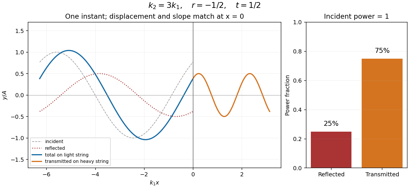
At the same tension, $k\propto \sqrt{\rho }$, so $k_2/k_1=3$, $t=1/2$ and $r=-1/2$. The transmitted power fraction is not $t^2$, because the two strings have different wave impedances. Using the energy flux of a transverse string wave,The reflected fraction is $\mathcal{R}=|r{|}^2=1/4$, so $\mathcal{R}+\mathcal{T}=1$. The transmitted displacement amplitude is $2.5\mathrm{mm}$ and its wavelength is $0.5/3\mathrm{m}$. The negative $r$ indicates a reflected phase reversal; it does not mean negative reflected energy.

Write the complex displacements as $y_1=(A{e}^{i{k}_{1}x}+B{e}^{-i{k}_{1}x})e^{-i\omega t}$ and $y_2=C{e}^{i{k}_{2}x-i\omega t}$. At a massless join, continuity of displacement and transverse force givesEliminating $B$ gives the displacement transmission coefficient and reflection coefficient,The angular frequency is shared across a stationary interface, whereas the wavelength changes. The equal-tension assumption is used in the slope condition.

Interpret the axis-directed route as successive coordinate-axis-parallel segmentsOn the first segment, $y=z=0$, so the field vanishes. On the second, $z=0$, so it again vanishes. On the last, $x=1$, $y=2$ and only $dz$ is nonzero, giving $\mathbf{F}\cdot d\mathbf{r}=8zdz$. ThusThe second and third segments are parallel to the corresponding global axes; they do not return to the global $y$- or $z$-axis before reaching the endpoint.

On the specified parametrized curve, $\mathbf{r}(t)=(t^2,2t,t^3)$ and ${\mathbf{r}}^{\prime }(t)=(2t,2,3t^2)$. Substitution into the field gives $\mathbf{F}(\mathbf{r}(t))=(4t^7,2t^8,8t^6)$. HenceThe line integral is thereforeBoth the field and the tangent vector must be evaluated along the curve; integrating one field component alone would miss two contributions.

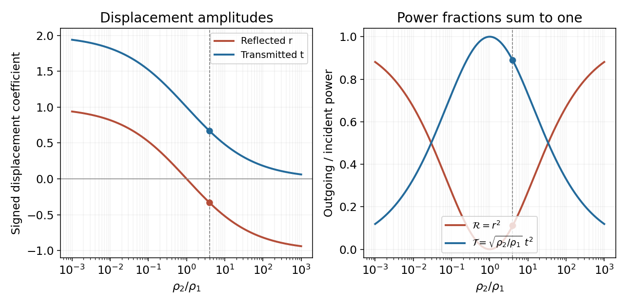
If ${\rho }_1\gg {\rho }_2$, then $k_1\gg k_2$ and the junction behaves approximately as a free end for the incident string. The limits areThe reflected displacement is not inverted, and at the junction it adds in phase to the incident displacement, producing nearly twice its amplitude. The transmitted displacement is also in phase. A transmission amplitude near two does not create power: the lighter string has much smaller impedance, and $\mathcal{T}=(k_2/k_1)t^2\simeq 4k_2/k_1\to 0$. These are limiting statements for positive densities, not an ordinary propagating-wave model for an exactly massless second string.

If ${\rho }_1\ll {\rho }_2$, then $k_1\ll k_2$ and the wave meets a much larger string impedance. The displacement and power coefficients approachThe junction behaves approximately as a fixed end. The reflected displacement reverses sign, corresponding to a phase shift of $\pi$; the small transmitted displacement is not inverted. For a large but finite density ratio, $t\simeq 2k_1/k_2$ and the transmitted power fraction is about $4k_1/k_2$, tending to zero rather than vanishing identically at every finite ratio.

For equal linear mass densities and common tension, $k_1=k_2$. The junction relations then giveThere is no mechanical-impedance discontinuity, so no reflected wave is needed to satisfy displacement and force continuity. The transmitted displacement is in phase with the incident wave and has the same amplitude; all incident power crosses the junction.

The reflected wave remains on the incident string, so its wavenumber magnitude is still $k_1$. Its outward power magnitude isThus $|P_r|+P_t=(1/9+8/9)P_i=P_i$, verifying energy conservation. With signed positive-$x$ fluxes, $P_r=-P_i/9$ and the same statement is $P_i+P_r=P_t$. The minus sign of the reflected displacement is a phase reversal, whereas the minus sign of its flux records travel in the opposite direction; these are different uses of a sign.

The transmitted and incident waves have the same angular frequency and tension, but the transmitted wavenumber is twice as large. The time-average string-power formula therefore givesThe extra factor $k_2/k_1$ is essential. Squaring the displacement transmission coefficient alone would give $4/9$, which is not the transmitted power fraction in strings with different linear mass densities.

With the same positive displacement convention for both masses, the first eigenvector equation is $(k+k_2-m{\Omega }^2)a_1-k_2{a}_2=0$. At the symmetric frequency it reduces to $k_2(a_1-a_2)=0$, while at the antisymmetric frequency it becomes $-k_2(a_1+a_2)=0$. HenceIn both normal modes the displacement magnitudes are equal. For the first, the masses move in phase and their separation stays unchanged; for the second they move in opposite phase, alternately approaching and separating. A negative signed amplitude ratio records a phase difference of $\pi$, not a negative displacement magnitude. The left panel of the later figure plots these signed normal mode shapes with the fixed wall values included.

Put $k_1=k_3=k$ and $m_1=m_2=m$. The mass-normalized stiffness matrix isIts symmetric eigenvector $(1,1)$ has eigenvalue $k/m$, while its antisymmetric eigenvector $(1,-1)$ has eigenvalue $(k+2k_2)/m$. ThusThe symmetric frequency does not depend on the middle spring constant because that spring has no extension in an in-phase normal mode. The antisymmetric motion stretches the middle spring and has the higher frequency for $k_2>0$.

Let $x_1,x_2$ be displacements from equilibrium, with positive directions chosen alike. Hooke's law and Newton's second law giveFor a normal mode $x_j=a_j\cos \Omega t$, the determinant condition isSolving the quadratic for ${\Omega }^2$ givesThe angular frequencies are the positive square roots. Positive masses and spring constants make the stiffness quadratic form $k_1{x}_1^2+k_2(x_2-x_1{)}^2+k_3{x}_2^2$ positive definite, ensuring both squared frequencies are positive. Distinct spring constants do not require equal masses or any symmetry approximation.

On $y=x$, the restricted function is $g(x)=2x^4-16x^2$. Its derivative is $g^{\prime }(x)=8x(x^2-4)$, so the turning points are $x=-2,0,2$. The restricted second derivative is $g^{\prime \prime }=24x^2-32$, negative at zero and positive at $\pm 2$. ThusThe corresponding points in the plane are $(0,0)$ and $(\pm 2,\pm 2)$. Along the diagonal the derivative is $f_x+f_y$, not a single arbitrary partial derivative; here $f_x=f_y$, so their zeros and sign changes agree with the restricted-curve calculation.

On $y=0$, the restricted function is $g(x)=x^4$, so $g^{\prime }(x)=4x^3$ changes from negative to positive at zero. HenceThe restricted second derivative vanishes there, but the quartic term determines the minimum. This does not contradict the two-dimensional saddle: values decrease along other directions, including the diagonal near the origin.

At an interior stationary point, a negative determinant of the symmetric Hessian matrix means its two eigenvalues have opposite signs. Along their eigenvectors the leading quadratic change has opposite signs, and the higher-order remainder cannot reverse these signs sufficiently close to the point. Hence the nondegenerate saddle condition isWhen the determinant vanishes, a saddle is still possible but is not determined by second derivatives alone: $x^4-y^4$ is a simple example. Thus these tests are decisive for nondegenerate stationary points, not an exhaustive classification from first and second derivatives of every smooth function.

At an interior stationary point, let $A=f_{xx}$, $B=f_{xy}$, $C=f_{yy}$ and $D=AC-B^2$. The quadratic change in the Taylor expansion is negative in every nonzero displacement when the Hessian matrix is negative definite. Applying the minimum test to $-f$ gives the sufficient nondegenerate maximum conditionsThe quadratic term then dominates the smaller Taylor remainder in a sufficiently small neighborhood, proving a strict local maximum. A vanishing determinant requires higher-order analysis instead.

For a twice continuously differentiable function, a finite second-order Taylor expansion about an interior point iswhere $A=f_{xx}$, $B=f_{xy}$, $C=f_{yy}$ at that point. A differentiable interior extremum requires $f_x=f_y=0$. For a strict minimum guaranteed by the quadratic term, the Hessian matrix must be positive definite. Completing the square gives $A{a}^2+2Bab+C{b}^2=A(a+Bb/A{)}^2+(AC-B^2)b^2/A$. Thus sufficient nondegenerate minimum conditions areIf $D=0$, the second-order test is inconclusive; for example $x^4+y^4$ has a strict minimum at zero despite a zero Hessian. The finite Taylor argument only needs $C^2$ regularity. The source's infinite Taylor representation additionally needs suitable analyticity: a smooth flat function, such as $e^{-1/(x^2+y^2)}$ extended by zero at the origin, has every Taylor coefficient zero there but is positive nearby.

For $z\ne -1$, multiply numerator and denominator by $\overline{z}+1$. The real part isThus its zero locus isIt is the unit circle with the point $-1$ removed. That point cannot be restored by the zero numerator obtained after clearing a denominator: the original expression is undefined there.