Subtract the two values of the survival function, or integrate the probability density function directly:The final zero records the requested third significant figure.

The survival function of this exponential distribution is $\mathbb{P}(T>t)=e^{-t/25}$ for $t\ge 0$. Therefore

Integrating the probability density function over the stated interval givesThe strict endpoint does not affect the probability for this continuous probability distribution.

At distance $x$ below the support, the cable must carry the weight of the remaining length $L-x$. Thus its equilibrium tension is $T(x)=\mu g(L-x)$, and the local transverse wave speed isThe linear mass density cancels. More precisely the small-displacement equation with variable tension is $\mu y_{tt}={\partial }_x[T(x)y_x]$; its local characteristic speed is the expression above, even though a first-spatial-derivative term is also present.

The wave travel time on a hanging uniform cable is obtained from $dt=dx/c(x)$:Although the local speed tends to zero at the free end, the endpoint singularity in the travel-time integral is integrable. This finite result belongs to the ideal flexible-cable model, with bending stiffness neglected.

Assume small transverse slopes, a flexible string, constant tension $T$ and uniform linear mass density $\rho$. For an element of equilibrium length $dx$, the vertical force is the difference of the vertical tension components at its ends. To first order in slope,Its mass is $\rho dx$ and its transverse acceleration is $y_{tt}$. Newton's second law therefore gives $\rho dx{y}_{tt}=Tdx{y}_{xx}$, orThis is the one-dimensional wave equation for small-amplitude transverse waves. Changes in string length and horizontal acceleration are second order in slope and are neglected in this linear approximation.

For $n=1$, the azimuthal unit vector is $\hat{\theta }=(-\sin \theta ,\cos \theta ,0)$, soOn a counterclockwise circle $C_r$ at fixed height, $dr=r\hat{\theta }d\theta$. Henceindependent of the positive radius. Clockwise orientation reverses the sign.

There is no contradiction with the zero curl found in solution. The vector field is undefined on the axis, so it is not continuously differentiable on a disc spanning $C_r$; the hypotheses of Stokes theorem fail for that disc. It is smooth on a planar annulus excluding the axis, where Stokes theorem correctly gives zero: the two boundary line integrals cancel, $2\pi -2\pi =0$.

The same check works for general $n$. A counterclockwise circle has circulation $\Gamma (r)=2\pi r^{2-2n}$. Integrating the curl over an annulus $a\le r\le R$ gives, for $n\ne 1$,For $n=1$, both sides are zero. Thus all three preceding results are consistent with Stokes theorem; the necessary distinctions are the regularity of the vector field and inclusion of every oriented boundary component.

In cylindrical coordinates, $F=r^{1-2n}\hat{\theta }$. The tangential coefficient is positive for every real $n$ and $r>0$, so the large-scale circulation is always counterclockwise when viewed from positive $z$.

By solution, the infinitesimal local angular velocity is $(1-n)r^{-2n}\hat{z}$. Its sign gives“Zero local spin” does not mean zero velocity: at $n=1$ a marked small element is still carried around the axis while its infinitesimal rotational component is zero. Orbital motion around the axis and local vorticity are different measurements.

Write $r^2=x^2+y^2$ and work away from the $z$ axis, where $r>0$. The vector field is independent of $z$ and has zero vertical component, so only the vertical curl can be nonzero:ThereforeThis local spin in an azimuthal power-law flow depends on the radial variation of the tangential speed, not merely on the sign of that speed.

Differentiate to obtain $g^{\prime }(y)=-1-4\sin y$. Let $\alpha =\arcsin (1/4)$, with $0<\alpha <\pi /2$. All solutions of $g^{\prime }=0$ areSince $g^{\prime \prime }(y)=-4\cos y$, the first family consists of local maxima and the second of local minima. Their function values follow from $4\cos \alpha =\sqrt{15}$:The derivative is periodic, but $g$ itself is not: increasing $y$ by $2\pi$ lowers $g$ by $2\pi$, which accounts for the indexed vertical offsets.

A stationary point is a point where the function is differentiable and its first derivative vanishes. Interpret the cube root as the real cube root, and put $q(x)=x^2-8x+7$. Then $f(x)=15+(x-3)\sqrt[3]{q(x)}$. For $x\ne 1,7$, the product rule and chain rule giveThe denominator is positive wherever it is defined. Consequently the two stationary abscissae areUsing the stationary equation to simplify the value of $q$ gives $q(x_{\pm })=-2(x_{\pm }+5)/5$. Thus the complete stationary points areNumerically they are approximately $(1.46762,17.10362)$ and $(6.13238,9.84664)$. The numerator of $f^{\prime }$ is positive outside $[x_{-},x_{+}]$ and negative inside, so the first is a local maximum and the second a local minimum.

At $x=1,7$, the real function is continuous but has a vertical tangent; the factor $x-3$ does not cancel either cube-root singularity. Those points are not stationary points. This is the distinction required when finding stationary points with real cube-root factors.

On an outward-oriented sphere of radius $R>0$, the electric field is normal with constant magnitude $A/R^2$. Thus its flux isIt is independent of $R$. There is no contradiction with solution: the classical divergence theorem cannot be applied to a full ball while pretending that $E$ is smooth at its center. On a punctured ball the outer flux and the inward-normal inner flux cancel, in agreement with zero ordinary divergence there.

The three-dimensional Dirac delta distribution ${\delta }^{(3)}(r)$ is supported at the origin and satisfies the sampling identityfor smooth compactly supported test functions $\phi$. It is not an ordinary function with a finite value at zero; its total integral is one, and translating it moves the point at which the test function is sampled.

The globally valid source equation isFor a direct weak verification, excise a ball of radius $\epsilon$ and integrate $-E\cdot \nabla \phi$ outside it. Since the ordinary divergence vanishes there, the result is $A{\int }_{S^2}\phi (\epsilon \hat{r})d\Omega \to 4\pi A\phi (0)$. This is precisely the displayed distributional divergence and restores the divergence theorem with the point charge included.

Away from the origin, the electric field is $E=Ar/r^3$, with $r$ here denoting the position vector in the numerator and its Euclidean norm in the denominator. The spherical-coordinate formula for divergence givesAt the origin the electric field is singular, so the ordinary divergence is undefined there. The equation above must not be extended to the whole space as an ordinary smooth-field identity. Its correct distributional divergence, derived in solution, includes the point source.

Take spherical polar coordinates with polar angle $\theta$ measured from positive $z$ and azimuthal angle $\varphi$:The derivative matrix isExpanding its determinant gives $r^2\sin \theta$. ThusThe inverse formula holds where $r>0$ and $0<\theta <\pi$; it excludes the origin and polar axis. These formulas use the general chain rule and determinant construction in solution.

For general coordinates $q=(a,b,c)$ expressed as functions of $u=(u,v,w)$, the chain rule gives $dq=Jdu$, whereThe Jacobian determinant is the oriented volume scaling of this linearized map. Thus the unsigned volume element transforms as $dadbdc=|\det J|dudvdw$. Where the coordinate change is invertible, the inverse Jacobian determinant is $1/\det J$, by the Jacobian chain rule.

For cylindrical coordinates, use $x=r\cos \varphi$, $y=r\sin \varphi$, and unchanged height $z$. Direct differentiation giveswhose determinant is $r$. ThereforeBoth directions are displayed because “from Cartesian to cylindrical” can refer either to the derivative of the new coordinates or to the factor used in transforming a Cartesian volume integral. They are reciprocals; the cylindrical axis is a coordinate degeneracy.

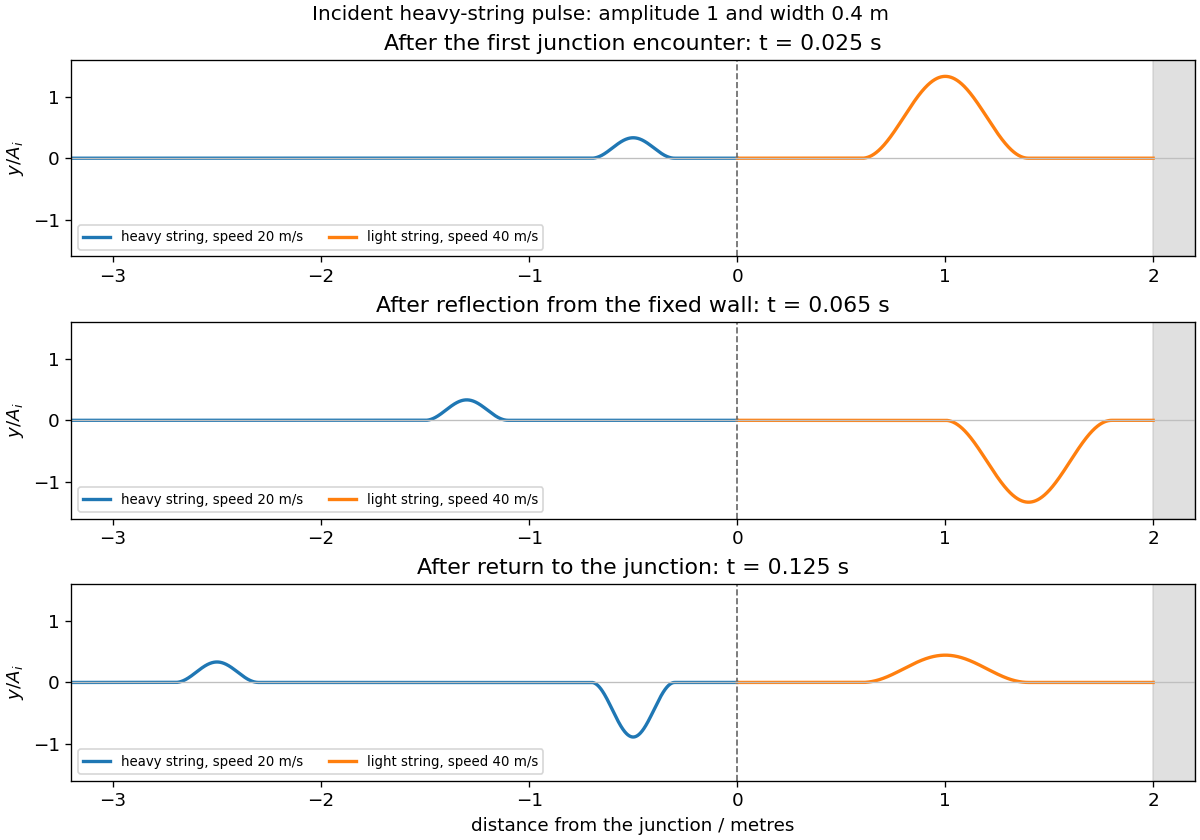
At the return encounter, transmission from light to heavy multiplies the amplitude by $2/3$, giving a backward heavy-string pulse of amplitude $-8A_i/9$. Its speed halves, so its width returns to $w$. Reflection within the light segment multiplies the incoming amplitude by $-1/3$, giving a right-going pulse of amplitude $4A_i/9$ and width $2w$. The earlier $A_i/3$ reflected pulse is already farther along the heavy string.

The sketches show these as separate pulses in the short-pulse regime $w/20\ll 0.10\mathrm{s}$. For longer pulses the corresponding components overlap and must be superposed rather than interpreted as isolated visible humps.

Reflection at a fixed end has displacement coefficient $-1$. The light-string pulse therefore returns from the wall with amplitude $-4A_i/3$ and width $2w$. It is inverted and travels left at $40\mathrm{m}{\mathrm{s}}^{-1}$. Taking the first junction encounter as time zero, its centre reaches the wall after $2/40=0.05\mathrm{s}$ and returns to the junction after $0.10\mathrm{s}$; a finite pulse takes its own duration to complete each encounter.

After the first encounter, the reflected pulse travels backwards through the heavy string with amplitude $A_i/3$ and width $w$. The transmitted pulse has amplitude $4A_i/3$ and speed $40\mathrm{m}{\mathrm{s}}^{-1}$. Its temporal duration is unchanged at the stationary junction, so its spatial width doubles to $2w$. Both pulses retain the original displacement sign.

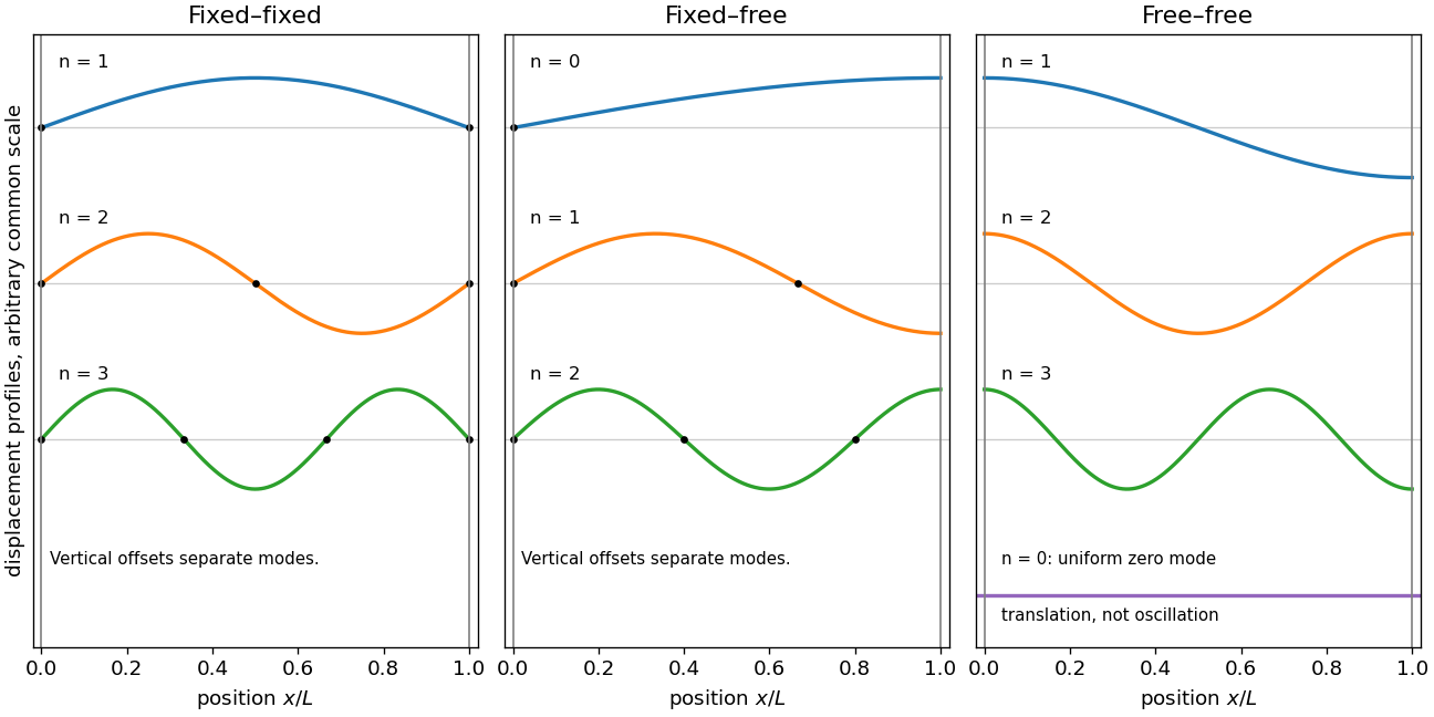
Free ends give $Y^{\prime }(0)=Y^{\prime }(L)=0$, so the oscillatory normal modes areThere is also the zero mode $k_0=0$, with uniform displacement $y_0(x,t)=a+bt$: a free string can translate without a restoring force. It is not a positive-frequency oscillation. The first three oscillatory shapes are $\cos (\pi x/L)$, $\cos (2\pi x/L)$ and $\cos (3\pi x/L)$, with an antinode at each end. The figure includes the uniform mode too, so that the zero-frequency limit is explicit.

A free end has zero transverse force, hence $T{Y}^{\prime }(L)=0$, rather than zero displacement. With $Y(0)=0$, write $Y=A\sin kx$. The remaining condition is $\cos kL=0$, givingThe first three shapes have one, three and five quarter-waves. Each has a node of a standing wave at the fixed end and an antinode at the free end; the mode frequencies are in the ratio $1:3:5$.

For a uniform string, let $c=\sqrt{T/\mu }$. A separated mode obeys $Y^{\prime \prime }+k^{2}Y=0$, $\omega =ck$. Fixed ends require $Y(0)=Y(L)=0$, soThe first three normal modes have one, two and three half-waves respectively. Their interior nodes of a standing wave are at $x=jL/n$ for $j=1,\dots ,n-1$.