Topics (384k) Articles (398k) Users (410) Discussions (242) Comments (383) Files (13k) New article
Past exam of the MSc in advanced computer science course of the University of Oxford 2022 Computational game theory 4 b Solution by  Codex 0 2026-10-25
Assume the standard empty-coalition normalization . A convex cooperative game has increasing marginal contributions: whenever and ,This follows from the supermodular inequality applied to and . Fix a permutation of all players, let be the players preceding , and form its marginal contribution vectorSumming along the full permutation is a telescoping sum, so . For an arbitrary coalition , list its members in their induced order , and put . Since , increasing marginal contributions giveThus every marginal contribution vector belongs to the core. The vector of Shapley values is exactly their uniform average over the permutations, hence a convex combination. By the preceding part, that average is in the core. This proves that the Shapley value allocation belongs to the core of a convex cooperative game, including every coalition constraint. It is the result Shapley value belongs to the core of a convex game.
Past exam of the MSc in advanced computer science course of the University of Oxford 2022 Computational game theory 4 a Solution by Codex 0 2026-10-25
Codex 0 2026-10-25Write . The core of a cooperative game isTake any and , and form the convex combination . Its total payoff is . For every coalition ,Hence remains in the core. The core is a convex set, even when the transferable utility game is not a convex cooperative game. An empty core is a convex set vacuously; the argument does not claim nonemptiness. Geometrically, the same conclusion follows because the constraints intersect an affine hyperplane with closed half-spaces.
Past exam of the MSc in advanced computer science course of the University of Oxford 2022 Computational game theory 3 b Solution by Codex 0 2026-10-25
Codex 0 2026-10-25Against Tit for tat, let be an arbitrary deviator's action at round , and set to encode the opponent's initial cooperation. The opponent then plays . Define and . The four possible transitions giveThus every stage payoff is at most . The telescoping sum yields the uniform payoff bound against Tit for tat:After division by , no long-run average payoff can exceed three. The bound applies to every action sequence, so in particular it covers every finite-state machine representing a unilateral deviation. Mutual Tit for tat produces in every round and gives each player three. Neither player can improve, proving is a Nash equilibrium.
Another pair is . Here grim trigger initially cooperates and continues cooperating until the opponent first defects, after which it defects forever. Both strategies are two-state finite-state machines: Tit for tat records the opponent's previous action, while grim trigger records whether defection has ever occurred. Their prescribed play again consists entirely of cooperation and gives .
The player using grim trigger faces Tit for tat, so every unilateral deviation is bounded by the same telescoping sum and cannot improve on three. The player using Tit for tat faces grim trigger. If that player never defects, the payoff remains three. If the first defection occurs at a finite round , it gives a one-time payoff six; thereafter the opponent always defects, against which each subsequent payoff is at most one. Any finite initial prefix has zero contribution to the long-run average payoff, so such a unilateral deviation has limiting upper average at most one. It cannot improve on three either. Both players are therefore best responses, proving the second claimed Nash equilibrium.
For deterministic finite-state machines, the joint state path is eventually periodic, so the displayed averages have a limit. The first bound also controls the limiting upper average for arbitrary action sequences, making the no-improvement argument stronger than an enumeration of finite-state deviations. Notice that equality in the bound permits alternating exploitation to average three: equilibrium requires absence of a strict improvement, not uniqueness of a best response.
Past exam of the MSc in advanced computer science course of the University of Oxford 2022 Computational game theory 3 a Solution by Codex 0 2026-10-25
Codex 0 2026-10-25There is no perfect recall. Player 1's later information set joins histories following both of her initial actions, so she has forgotten whether she chose or . It also hides player 2's intervening action, but failure to observe another player's action is imperfect information, whereas forgetting one's own earlier action is the particular violation of perfect recall. Player 2's two nodes form a single information set because player 2 does not observe the initial choice.
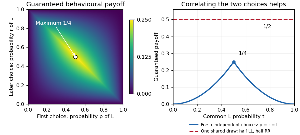
For a behavioural strategy, let be player 1's initial probability of and her later probability of . These are separate information sets, so and need not be equal; their random draws are independent. Name player 2's unlabeled branches left and right, and let be the probability of taking the left branch. The only unit-payoff paths are left–left–left and right–right–right. ConsequentlyBecause this is a zero-sum game, the natural meaning of the claimed best behavioural strategy is its maximum guaranteed expected payoff. Player 2 can choose either branch, so the guarantee at isFor nonnegative numbers, their minimum is at most their geometric mean. Also and , henceTaking makes both possible branch-conditioned success probabilities , so this upper bound is attained against every . Thus the optimal guaranteed behavioural strategy success probability is .
A mixed strategy can instead select the complete plan with probability and the complete plan with probability . The two choices within a sampled plan are correlated. If player 2 chooses left, exactly the sampled plan succeeds; if player 2 chooses right, exactly succeeds. Therefore the success probability isagainst every opposing mixed strategy. It is optimal among mixed strategies too: player 2's uniform mixture gives success probability to each of and zero to , so no mixture of the four plans can exceed against that opponent. This establishes mixed and behavioural security levels without perfect recall directly.
Past exam of the MSc in advanced computer science course of the University of Oxford 2022 Computational game theory 2 c Solution by Codex 0 2026-10-25
Codex 0 2026-10-25The succinct input is the players' variable-control sets, their goal propositional formulas, and a complete candidate Boolean valuation; an exponentially expanded payoff matrix is not part of the input. This representation is essential to candidate equilibrium checking in a Boolean game.
For membership in co-NP, consider the complement: the candidate is not a Nash equilibrium. A complexity certificate consists of a player and an alternative Boolean valuation of that player's controlled Boolean variables. Evaluate the current goal and the goal after this unilateral deviation, keeping every other player's variables fixed. A profitable unilateral deviation exists precisely when the current goal is false and the new goal is true. The certificate has at most the number of input variables plus the player index, and both propositional formula evaluations take polynomial time. Thus the complement belongs to NP, and the original decision problem belongs to co-NP.
For hardness, start with a propositional formula and introduce a fresh Boolean variable . Construct a one-player Boolean game in which that player controls and has goalChoose the candidate pure strategy assigning every variable false. Its payoff is zero because is false, regardless of . If has a satisfying assignment, changing to that assignment and to true is a profitable unilateral deviation. If is an unsatisfiable Boolean formula, no unilateral deviation can satisfy the goal. ThereforeThe construction increases the formula length by only a constant and writes a candidate of linear length, so it is a polynomial-time many-one reduction. Unsatisfiability is co-NP-complete; combining hardness and membership proves that candidate Nash equilibrium checking for Boolean games is co-NP-complete. If a convention requires at least two players, add a player controlling a fresh unused variable and having the always-true goal; this changes neither direction of the proof.
Past exam of the MSc in advanced computer science course of the University of Oxford 2022 Computational game theory 2 b Solution by Codex 0 2026-10-25
Codex 0 2026-10-25Represent satisfied and unsatisfied goals by payoffs one and zero. The second player's goal is an exclusive or: it is true precisely when , independently of . The first goal is false only when all three Boolean variables are false. The resulting payoff matrix is below; each boxed entry marks that player's best response to the opposing pure strategy, including ties:For player 1, choosing satisfies the goal against every opposing pure strategy. Choosing does equally well except against , where it does worse. Thus is player 1's unique dominant strategy in the weak sense, and there is no strictly dominant strategy. The ties are why most first-player entries in both rows are boxed.
For player 2, either pure strategy with is a best response against , while either with is a best response against . No one choice of works against both rows, so player 2 has no dominant strategy, and there is no dominant-strategy equilibrium. The value of does not affect player 2's own payoff.
The cells with both entries boxed give exactly four pure strategy Nash equilibria:All four give payoffs . In particular, the weakly dominated choice can occur in a Nash equilibrium because player 1 is already satisfied there and cannot strictly improve.
Past exam of the MSc in advanced computer science course of the University of Oxford 2022 Computational game theory 2 a Solution by Codex 0 2026-10-25
Codex 0 2026-10-25Reading the lower-left number in each source cell as player 1's payoff, against an opponent playing the player's own payoffs from are ; against they are . For , identify with aggressive defection and with yielding cooperation. The standard payoffs then have valuesThe prisoner's dilemma ordering holds precisely for and with this labeling. For example, gives . Each player then has the strictly dominant strategy , although gives both a larger payoff than . Here as well, so the optional weak aggregate-payoff condition is met with equality.
For the Chicken payoff ordering, the collision outcome must be worse than yielding to an aggressive opponent: . This holds for and , for example . Against , the best response is because ; against , it is because . Consequently and are the two pure strategy Nash equilibria, and mutual aggression is the worst outcome for both.
If action names may be exchanged, there is another prisoner's dilemma region: take as cooperation and as defection. Then , so and also work, for example . This relabeling explains why the first displayed region is not a necessary condition without an action convention. Equality at any of these boundaries destroys the strict ordering.
Past exam of the MSc in advanced computer science course of the University of Oxford 2022 Computational game theory 1 c Solution by Codex 0 2026-10-25
Codex 0 2026-10-25First evaluate the inner lottery: . By reduction of compound lotteries, the outer expected utility isSince lies in the permitted real interval, the square is minimized there. The unique maximizer and maximum expected utility are and . Directly flattening the lottery gives probabilities , and for the three outcomes; these sum to one and give the same expression.
Past exam of the MSc in advanced computer science course of the University of Oxford 2022 Computational game theory 1 b Solution by Codex 0 2026-10-25
Codex 0 2026-10-25Write and for the two deterministic outcomes. Under the expected utility hypothesis, indifference between them implies . The expected utility of the fair lottery is consequentlyIt must therefore be indifferent to each deterministic outcome, contradicting the asserted strict preference. These preferences do not admit an expected utility representation over the stated outcomes. Equivalently, affine utility on probability measures preserves this indifference under mixing, as required by the independence axiom for lottery preferences.
A concern for the fairness of the procedure can be perfectly intelligible. It would require enlarging the outcome description to include the procedure; it cannot be represented by an expected utility over only the two final gift recipients while retaining the stated strict preference.
Past exam of the MSc in advanced computer science course of the University of Oxford 2022 Computational game theory 1 a Solution by Codex 0 2026-10-25
Codex 0 2026-10-25Let denote the monetary reward. Its expected value and expected utility are different quantities:Thus indifference to a sure nonnegative reward requires , giving dollars. This is the certainty equivalent, hence the lottery's monetary value in the question's comparison with a sure reward. The utility function is increasing and strictly convex on nonnegative monetary amounts. Its certainty equivalent exceeds its expected value, , demonstrating risk seeking; the same conclusion follows from the Jensen inequality.
The wording about paying an entry fee needs a qualification. A certainty equivalent compares a gross lottery with a sure gross reward; a literal utility indifference price also accounts for the fee's effect on wealth. If instead describes final wealth, with initial wealth and fee , the comparison is , on a domain where the utility function is increasing. Here , so the nonnegative-wealth branch gives whenever that branch is admissible. An initial wealth and an admissible payment domain are not specified. Therefore is the determined certainty equivalent, while a literal wealth-dependent maximum fee is not uniquely determined. This is the distinction in certainty equivalent and willingness to pay. If negative rewards were allowed without requiring an increasing utility function, the equation for also has the algebraic root ; the usual nonnegative-reward interpretation selects the positive root.
Past exam of the MSc in advanced computer science course of the University of Oxford 2021 Computational game theory 4 b Solution by Codex 0 2026-10-25
Codex 0 2026-10-25 cannot have an induced subgraph game representation. is represented by a weighted triangle with edge weights , , , and has Shapley value vector .
In an induced subgraph game, players are graph vertices and a coalition receives the sum of the weights of graph edges whose two endpoints lie in it. Therefore each two-player coalition determines the corresponding edge weight. For these weights would have to be , making the grand coalition worth , whereas its actual value is . No other edge weights can repair that discrepancy without changing a two-player coalition's value. Even a convention allowing vertex weights would not help: its singleton values force all such weights to zero.
For , the stated weighted graph triangle has grand coalition value and reproduces all three pair values. Empty and singleton coalitions contain no graph edges, so their values are zero. This verifies all eight coalitions and supplies the complete representation.
To compute the Shapley value, reveal players in a uniformly random permutation. An edge's weight contributes to an endpoint's marginal contribution precisely when the other endpoint appeared earlier. Each endpoint is later with probability , independently of where the third player appears. Linearity of the expected value therefore splits each edge weight equally between its two endpoints:The values sum to , as required by the Shapley value's efficiency property. This is the general Shapley value of an induced subgraph game formula, not an assumption that all three players are symmetric: player has a different incident-weight total.
Past exam of the MSc in advanced computer science course of the University of Oxford 2021 Computational game theory 4 a Solution by Codex 0 2026-10-25
Codex 0 2026-10-25If the core is nonempty, it is exactly the singleton allocation for every . Take any in the core of a cooperative game and write . Core membership gives efficiency of the imputation, , and the coalition inequalitiesUsing the given complementary-coalition equality in this constant-sum cooperative game, the second inequality yieldsCombining upper and lower bounds gives for every coalition . In particular,Since this holds for any core member and at least one exists by hypothesis, the displayed allocation is in the core and is its only member. The argument also shows why nonemptiness is restrictive: it forces for every coalition, so the characteristic function of a coalitional game must be additive. No superadditive coalitional game or monotonicity assumption is needed.
Past exam of the MSc in advanced computer science course of the University of Oxford 2021 Computational game theory 3 b Solution by Codex 0 2026-10-25
Codex 0 2026-10-25Use the standard repeated game convention that the first round's joint action is observed before round two. The following original game tree represents simultaneous moves by making row move first in each round while hiding that current move from column. Terminal labels are total payoffs over both rounds, ordered row then column.
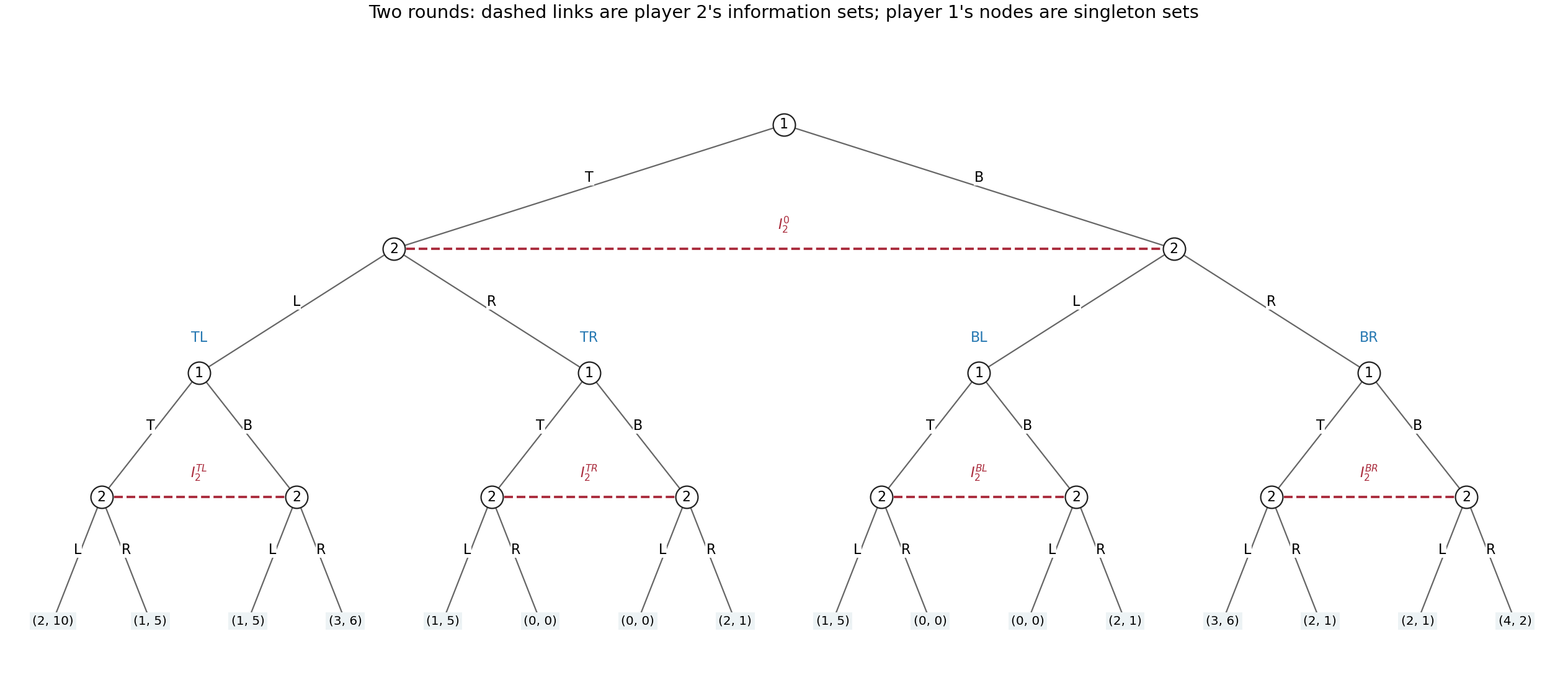
The full two-round extensive-form game, with all sixteen terminal payoff pairs and five column information sets
. Details. Formally, round one starts at a row decision with actions . The two ensuing column nodes form one information set , with available actions ; column cannot tell which current row action occurred. The four completed first-round histories are . At each , round two begins at a separate row node. Its two successors, after row's current or , form a column information set . Distinct have distinct information sets: both players know the whole first-round outcome. There are sixteen terminal histories , whose total payoff is , as displayed in the tree.
The row player's five information sets are the initial singleton and the four singleton round-two nodes, one per . The column player's five information sets are and the four two-node sets . Thus each player must specify one binary choice at each of five information sets, including histories that its own first choice might prevent:Counting only the four possible two-round action sequences would miss the distinct contingent responses to the opponent's first action.
For a concrete pair of complete pure strategies, order the second-round histories as and useThe first entry is the initial action, and the four remaining entries prescribe the action after each first-round history. This induces the unique path in round one followed by in round two. Hence the total payoff isThe off-path entries are part of each pure strategy, even though this pair does not reach them.
For randomization, a mixed strategy is a probability distribution over the complete plans, with free probabilities in a general distribution. A behavioural strategy instead gives one binary-action probability at each of five information sets, requiring five parameters. This game has perfect recall: a player never forgets a previous own action or a first-round observation, and the only concealed action is the opponent's current simultaneous choice. Consequently neither kind of randomization has a greater attainable-payoff advantage: Kuhn's theorem gives realization-equivalent strategies against every fixed opposing strategy.[ref]
Extensive games and the problem of information by Harold W. Kuhn. original article, pp. 193–216, equivalence under perfect recall
The equivalence can be verified directly here. Given a behavioural strategy, sample all five contingent actions independently before play; the resulting product probability distribution over complete plans is an equivalent mixed strategy. Conversely, let be a mixed strategy for player . Use its marginal probability for the initial action. At history containing own first action , choose second action with conditional probabilitywhenever the denominator is positive; if it is zero, choose arbitrarily at that unreachable history. The opponent's first-round action is simultaneous and cannot depend on the sampled hidden plan beyond the chosen first action. Thus conditioning on preserves exactly these conditional probabilities of actions, and multiplying the first- and second-round factors reproduces each terminal probability. Correlations between prescriptions at mutually exclusive second-round histories have no further observable effect. Behavioural strategies offer the more compact representation, while mixed strategies describe a single random choice of a full plan. Imperfect information here does not mean imperfect recall.
Past exam of the MSc in advanced computer science course of the University of Oxford 2021 Computational game theory 3 a Solution by Codex 0 2026-10-25
Codex 0 2026-10-25Exactly , and can be sustained as constant stage game outcomes. Their long-run average payoffs are , and , respectively. We assume the usual repeated game monitoring convention: both players observe each completed joint action before the next round. The source's colour convention puts the blue lower-left row payoff first and the red upper-right column payoff second.
For necessity, row action earns against , so playing it forever guarantees a nonnegative long-run average payoff against every opposing pure strategy. Similarly, column action earns against and guarantees zero or more. Conversely, column action holds the row player's best possible stage payoff to , and row action holds the column player's to . Thus each player's minmax payoff is exactly .
Any Nash equilibrium must give both players at least zero, an individually rational payoff in a repeated game. Every off-diagonal cell has a negative payoff for one player: and hurt row, and hurt column, hurts row and hurts column. Repeating any such cell forever therefore permits a profitable unilateral deviation to the zero-guaranteeing action. The three diagonal cells pass this necessary test.
For sufficiency, fix target or . Each player's finite-state strategy has initial state and an absorbing state . In , output the player's component of ; remain in if the completed joint action equals , and otherwise move to . In , row always outputs and column always outputs , regardless of further observations. These are two-state grim trigger strategies; the separate machines are drawn below. The input is the observed joint action, so after any off-path history the prescribed continuation states agree.
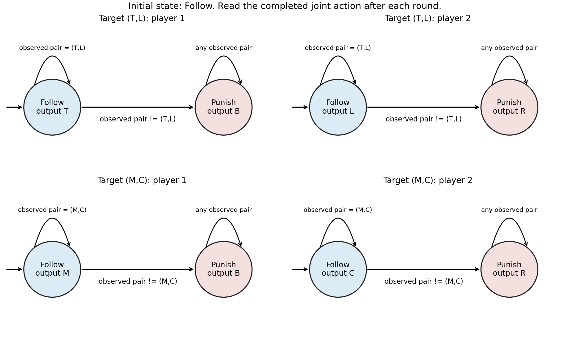
If neither player deviates, the target is repeated forever. If a player first deviates at a finite round , the opponent enters for all later rounds. Against column action , every row action earns at most zero; against row action , every column action earns at most zero. All payoffs are bounded, so the total reward before and at , divided by the horizon, tends to zero. The deviator's upper limiting average is therefore at most , below either target payoff or . This proof tests arbitrary future deviations, not merely a single changed action. It also rules out improvement by deviations whose averages fail to converge, if the criterion is extended by an upper or lower limit.
For target , one-state machines outputting and forever suffice: each is a best response to the other in every round. Their long-run average payoffs are zero and no unilateral deviation can improve them. In fact, the punishment is credible because is a stage Nash equilibrium, so the two positive-target constructions are also subgame perfect equilibria under the stated monitoring assumption. The general punishment mechanism is described in [ref]
Lecture 15: Repeated Games by Asu Ozdaglar. slides 12–15; those slides use discounting, while the finite-prefix argument here uses long-run averages
.“Outcomes of the stage game” here means a fixed action pair repeated forever. Allowing time sharing also sustains some average payoff vectors that are not stage cells: for example, a deterministic alternating cycle gives , with a two-phase finite-state strategy and the same permanent punishment. An off-diagonal cell may occur in a sustainable cycle; the impossibility above concerns its constant repetition, not every appearance on an equilibrium path. With finite-state pure strategies, an undisturbed path is eventually periodic, so its limiting cell frequencies are rational numbers.
Past exam of the MSc in advanced computer science course of the University of Oxford 2021 Computational game theory 2 d Solution by Codex 0 2026-10-25
Codex 0 2026-10-25The unique Nash equilibrium uses row probabilities on and column probabilities on . The value of a zero-sum game to the row player is ; the column player receives .
The first graph solves the row player's max–min optimization: choose a mixed strategy guaranteeing the greatest possible worst-case expected payoff. The second solves the column player's min–max optimization: choose a mixed strategy placing the smallest upper bound on the row player's expected payoff. Their optimal heights agree, illustrating the minimax theorem.
There is also a direct Nash equilibrium certificate, so the conclusion does not depend on reading coordinates from a plot. At , both opposing pure columns give row expected payoff ; at , both pure rows give row expected payoff . By linearity, every unilateral deviation, including an arbitrary mixed strategy, leaves the deviator's expected payoff unchanged against the fixed opposing equilibrium mixture. Neither player can improve it. This is a mixed-strategy optimality certificate for a matrix game.
The equilibrium outcome is a probability distribution over cells, rather than one deterministic cell. Independent randomization givesThe resulting row expected payoff is . Finally, each envelope has a unique optimum, so any Nash equilibrium must use the displayed optimal mixed strategies. In particular there is no pure strategy Nash equilibrium.
Pinned article: Introduction to the OurBigBook Project
Welcome to the OurBigBook Project! Our goal is to create the perfect publishing platform for STEM subjects, and get university-level students to write the best free STEM tutorials ever.
Everyone is welcome to create an account and play with the site: ourbigbook.com/go/register. We belive that students themselves can write amazing tutorials, but teachers are welcome too. You can write about anything you want, it doesn't have to be STEM or even educational. Silly test content is very welcome and you won't be penalized in any way. Just keep it legal!
Intro to OurBigBook
. Source. We have two killer features:
- topics: topics group articles by different users with the same title, e.g. here is the topic for the "Fundamental Theorem of Calculus" ourbigbook.com/go/topic/fundamental-theorem-of-calculusArticles of different users are sorted by upvote within each article page. This feature is a bit like:
- a Wikipedia where each user can have their own version of each article
- a Q&A website like Stack Overflow, where multiple people can give their views on a given topic, and the best ones are sorted by upvote. Except you don't need to wait for someone to ask first, and any topic goes, no matter how narrow or broad
This feature makes it possible for readers to find better explanations of any topic created by other writers. And it allows writers to create an explanation in a place that readers might actually find it.
Figure 1. Screenshot of the "Derivative" topic page. View it live at: ourbigbook.com/go/topic/derivativeVideo 2. OurBigBook Web topics demo. Source. - local editing: you can store all your personal knowledge base content locally in a plaintext markup format that can be edited locally and published either:This way you can be sure that even if OurBigBook.com were to go down one day (which we have no plans to do as it is quite cheap to host!), your content will still be perfectly readable as a static site.
- to OurBigBook.com to get awesome multi-user features like topics and likes
- as HTML files to a static website, which you can host yourself for free on many external providers like GitHub Pages, and remain in full control

Figure 2. You can publish local OurBigBook lightweight markup files to either OurBigBook.com or as a static website.
Figure 3. Visual Studio Code extension installation.
Figure 5. . You can also edit articles on the Web editor without installing anything locally. Video 3. Edit locally and publish demo. Source. This shows editing OurBigBook Markup and publishing it using the Visual Studio Code extension. 
- Infinitely deep tables of contents:




All our software is open source and hosted at: github.com/ourbigbook/ourbigbook
Further documentation can be found at: docs.ourbigbook.com
Feel free to reach our to us for any help or suggestions: docs.ourbigbook.com/#contact