The TeX input processor converts input characters into TeX tokens using their current TeX category codes. Its whitespace handling is described by TeX input states: new line N, skipping spaces S and middle of line M.^[ref]

Under ordinary conventions, the invented input A B produces an A character token, one space token and a B character token. After A, state M allows the first space through and switches to S; the next two spaces disappear. Reading B returns to M. A space-only line begins in N and its end produces \par, whereas the end of an ordinary text line in M supplies a space.^[ref]

This explains why source indentation and repeated spaces need not survive as visible word spacing. The complete scanner also handles comments, TeX control sequences and character-code conversions; the N/S/M diagram describes the whitespace part of the process.

Radio tracking estimates the location or movement of a target using radio waves associated with it. In a basic beacon system, a radio transmitter travels with the target while a radio receiver and directional antenna provide observations from known positions. An audible received pulse can identify a transmitter and help determine its direction; it does not itself supply map coordinates.^[ref]

Radio direction finding can be combined across stations by radio triangulation. In a hypothetical horizontal Cartesian coordinate system, station $A=(0,0)$ finds a target along $y=x$, while station $B=(2,0)$ finds it along $y=2-x$, with distances in kilometres. The intersecting forward bearings give $(1,1)$. A single bearing instead leaves many possible positions along one direction. Nearly parallel bearings constrain the intersection poorly: a small angular error can then produce a large position error.

A field example is local bird tracking described by the Smithsonian Migratory Bird Center. Researchers use received signals to follow a tagged bird or combine directions from different observation points, allowing repeated observations without continuous visual contact. Receiver range, battery life and the placement of observing stations limit which movements are recorded. A missing signal therefore need not mean that the animal stopped moving or died; it may have moved beyond detection.^[ref]

A taxonomic family is a taxonomic rank above a genus and below a taxonomic order. A particular family is a named group of organisms placed at that rank; the rank itself is a position in the classification hierarchy.^[ref]

For example, the cat family Felidae includes the genera Felis and Panthera. The family groups several genera, while each genus groups species. Scientific classifications draw on morphological, molecular and other evidence when deciding which organisms belong together.^[ref]

A constructed counting example separates hierarchy from abundance. If a hypothetical family contains two genera with three and five recognized species respectively, it contains eight species, provided those lists are disjoint and complete. It need not contain eight individual animals: the same eight species could be represented by millions of organisms.

The rank does not prescribe a fixed number of genera or species. Nor is a family label itself a measurement of evolutionary time. A phylogenetic tree represents hypotheses about ancestry and branching; ranked names organize those organisms at selected hierarchical levels. Changes in evidence can lead to revised membership without changing what the rank word means.^[ref]

A taxonomic rank is a named level in a biological classification hierarchy. Taxonomic order, taxonomic family, genus and species are ranks; Carnivora is a taxon at order rank, and Felidae is a taxon at family rank. A rank answers what level a group occupies, while a taxon identifies which group is meant.^[ref]

In a simplified nested classification, let $S$, $G$, $F$ and $O$ be the organism sets belonging to one species, its genus, its family and its order. Then $S\subseteq G\subseteq F\subseteq O$. The subset symbol expresses inclusion, not equality of the number of members or a fixed numerical spacing between levels.

For instance, a hypothetical family can contain one genus with ten species, whereas another family contains five genera with two species each. Both have ten species and occupy the same rank, yet their internal grouping differs. Rank, species count and genus count are distinct data.

Nor must each biological clade receive a traditional rank: a phylogenetic tree can resolve many branching groups between two named levels. The hierarchy provides a practical naming framework, while the evolutionary hypothesis contains additional structure.^[ref]

A taxonomic order is a taxonomic rank below a taxonomic class and above a taxonomic family. An order is a named grouping, or taxon, at that position in a classification. Its constituent families can themselves contain several genera and species.^[ref]

For example, Carnivora is an order containing the cat family Felidae. The order name and family name identify groups at different levels; the same animal belongs to both. This is nested classification rather than two competing identifications.^[ref]

A constructed database example illustrates the information lost during aggregation. Suppose an order contains three families with 2, 4 and 1 sampled species respectively. Reporting seven species for the order preserves the total but discards how those records were distributed among families. An analysis at order level can therefore conceal variation visible at family level.

The rank specifies hierarchical placement, not a fixed age, number of species or amount of genetic divergence. A phylogenetic tree instead expresses a hypothesis about ancestry and branching. Classification uses evolutionary evidence, but a rank label alone is not a numerical evolutionary distance.^[ref]

A taxonomic class is a taxonomic rank conventionally below a taxonomic phylum and above a taxonomic order. A particular class is a taxon at that level. For example, Mammalia is the class of mammals, and Carnivora is one of its constituent orders.^[ref]

The hierarchy makes several statements simultaneously: an individual cat belongs to Mammalia, Carnivora and Felidae, at class, order and family ranks respectively. These nested memberships describe increasing specificity. They do not give three independent estimates of the cat's identity.

Consider a constructed sampling table with two classes, each represented by twelve sampled species. The first has two sampled orders containing six species each; the second has three containing four each. The class totals agree, while the within-class distribution differs. Class-level aggregation preserves the total and discards that structure. Nor would twelve sampled species establish twelve species in the complete class: sampling coverage is a separate issue.

A taxonomic class need not have a fixed number of orders, individuals or species. Its rank also does not specify a fixed age or a numerical amount of genetic divergence. Those are additional biological quantities or hypotheses that require evidence beyond the hierarchical label.

A taxon is a group of organisms recognized as a unit in taxonomy. A taxonomic rank specifies a position in the classification hierarchy; a taxon is the particular group placed there. Thus Felidae is a taxon at the rank of taxonomic family, while Carnivora is a taxon at the rank of taxonomic order.^[ref]

One organism can belong to many nested taxa. Membership in a species, its genus and its taxonomic family describes different levels of the same classification. A rank alone does not identify the group: the word family could refer to many distinct taxa.

For a constructed information-system example, let a family contain genera A and B, with three and five recognized species respectively. A species record can store its species identifier and follow parent relationships to recover its genus and family. If a later classification moves one species from A to B, the family's species total remains eight, while the genus totals change from 3 and 5 to 2 and 6. Group membership and the name of the rank are separate pieces of information.

A clade is specifically a group containing an ancestor and all its descendants. Calling a group a taxon does not by itself establish that it is a clade; that claim depends on its circumscription and the inferred phylogenetic tree.^[ref]

A taxonomic phylum is a major taxonomic rank conventionally below a taxonomic kingdom and above a taxonomic class. A particular phylum is a taxon at that rank. For example, chordates form the phylum containing Mammalia, which in turn contains orders such as Carnivora.^[ref]

The same animal can consequently belong to a phylum, a class and an order without these being competing identifications. Each level adds information about nested membership. The rank word phylum identifies a position in the hierarchy; the group name identifies which taxon occupies that position.

For a constructed survey example, suppose one phylum is represented by four sampled classes with 3, 7, 2 and 8 sampled species. Its total is $3+7+2+8=20$. A second phylum with two sampled classes containing ten species each has the same total. Reporting only twenty species for each phylum loses the class-level distribution, and neither count establishes the total diversity of the unsampled phylum.

A taxonomic rank does not itself specify a fixed age, number of constituent groups or numerical genetic distance. A phylogenetic tree addresses evolutionary relationships, while ranked names select particular groupings for classification.^[ref] The usefulness of the rank comes from organizing comparisons; the scientific interpretation still depends on what was sampled and the evidence supporting membership.

A taxonomic kingdom is a major taxonomic rank conventionally below a domain and above a taxonomic phylum. A kingdom is a particular taxon at that rank, while the rank word identifies its place in a classification. In a familiar classification of eukaryotes, animals and plants belong to different kingdoms within the same domain.^[ref]

Nested membership permits several descriptions of one organism. An individual animal can belong to the eukaryotic domain, the animal kingdom and a particular phylum simultaneously. The levels select different scales of grouping, rather than offering competing identifications.

A constructed classification database illustrates the information supplied by parent relationships. Suppose kingdom A contains phyla P and Q, with 8 and 12 recorded species, while kingdom B contains phylum R with 20 recorded species. Both kingdom totals are twenty, but A's records are divided between two phyla and B's are not. A query grouped only by kingdom loses that distribution. The counts describe the stipulated records, not a census of complete biological diversity.

The kingdom rank does not prescribe a fixed number of phyla or a particular evolutionary age. Nor does sharing that rank establish equal evolutionary distance between any two groups. A phylogenetic tree represents hypotheses about ancestry and branching; a ranked classification assigns names to selected groupings.^[ref] Keeping the rank, the membership and the supporting evidence separate makes comparisons across classifications more interpretable.

A type species is the species serving as the nomenclatural type of a genus under a naming code that uses this form of typification. It anchors application of the genus name. It is not necessarily an average, an ancestor or the most familiar member of the genus.

In prokaryotic nomenclature, the Code explicitly identifies the type of a genus or subgenus with a type species and specifies how that species is fixed. If a genus originally included only one species when validly published, that species is its type even without an explicit designation. These are naming rules, not measurements of evolutionary distance.^[ref]

An original hypothetical example separates the reference from a summary statistic. Suppose a genus contains species T, U and V, with T the designated type species. A measured trait has values1,10 and11, whose arithmetic mean is $22/3\approx 7.33$. U lies nearer that mean, but this does not make U the type. The designation and the statistical comparison answer different questions.

Now suppose new evidence from phylogenetics divides the hypothetical group into T+U and V. The existing reference is associated with the group containing T; how the remaining group is named requires the relevant naming rules and publication history. Merely discovering that V has an unusual trait does not transfer the reference to it.

The anchor has another level beneath it. In the ordinary prokaryotic case a species itself has a type strain, whereas the genus has a type species. A stored culture accession, a species reference and a genus reference therefore do not all denote the same rank or the same physical object.^[ref]

A type species stabilizes the connection between a name and its reference while taxonomy remains open to revised evidence. The detailed code governing the organisms concerned must be stated; one nomenclatural example should not silently impose every prokaryotic rule on other branches of biology.

A macromolecular structural model is a representation of the three-dimensional organization of a biological macromolecule or complex. It can include atom identities, coordinates, crystallographic site occupancy, atomic displacement parameters and alternative conformations. A deposited coordinate set is an interpreted model supported by measurements, rather than the measurements themselves.^[ref]

For X-ray crystallography, an electron density map constrains where atoms can be placed, while chemical geometry and experimental uncertainty constrain interpretation. Poorly resolved regions can remain absent from the model or be represented less precisely. A numerical coordinate printed to several decimal places does not establish equally fine positional accuracy.

An original coordinate comparison illustrates the distinction. Suppose two models place the same atom at $(0,0,0)$ and $(0.2,0,0)$ in angstrom units. Their separation is $0.2\mathring{\mathrm{A}}$, but that number alone cannot say which model is better. One must examine agreement with the data and the relevant uncertainty, not merely the number of digits or the difference between the coordinates.

A concrete example is calmodulin structure1CLL in the Protein Data Bank. The record contains a refined model with four calcium ions, while its primary citation describes poorly defined terminal residues. Both the observed binding environment and the unresolved regions are part of interpreting the structure.^[ref]

Structural claims should therefore specify which components and conformations are modeled, what experiment supports them and what remains unresolved. A model useful for one question does not automatically establish the complete dynamics or every biochemical activity of the molecule.

Stereo disparity is the difference between the image positions of the same scene feature in two views. For an ideal horizontally aligned pair, use signed horizontal coordinates with matched principal points and defineWith the orientation and camera baseline convention of stereoscopic triangulation, a point in front of the cameras has $d=fB/Z$: stereo disparity measures inverse depth, rather than depth itself. Halving $d$ doubles $Z$ when the camera baseline and focal length stay fixed.

A disparity map assigns this difference to matched image locations. Finding the matches is a separate stereo correspondence problem. A repeated pattern can give several plausible matches; a feature hidden from one camera has no visible partner. A small measured stereo disparity is therefore not, by itself, proof of a distant object: the match and calibration must also be credible.^[ref]

The ideal relation also explains why far-away reconstruction becomes sensitive to measurement error. Differentiating $Z=fB/d$ gives $\mathrm{d}Z/\mathrm{d}d=-fB/d^2$; the first-order propagation of uncertainty is ${\sigma }_Z\simeq fB{\sigma }_d/d^2$. Thus equal disparity errors produce larger depth errors at greater depth. The example and curves under stereoscopy quantify this effect.

Stereoscopic triangulation reconstructs a scene point from corresponding image positions and known camera geometry. Each image position determines a viewing direction. Two correctly matched views constrain the point to lie on both viewing rays; one view alone leaves its position along a ray undetermined.

For an ideal aligned pair, put the left camera at the origin and the right one at $(B,0,0)$ in a Cartesian coordinate system, with their axes pointing in the positive $Z$ direction. Assume a common focal length $f$, square pixels, corrected distortion and image coordinates measured from aligned principal points. Forward perspective projection givesThe stereo disparity $d=u_L-u_R$ therefore determines all three coordinates:Here $Z$ is depth along the camera axis; the Euclidean distance from the left camera is instead $\sqrt{X^2+Y^2+Z^2}$. If $f,u_L,v_L,d$ use pixels and the camera baseline $B$ uses metres, the recovered coordinates use metres. Without a known length scale, the images alone do not determine metric size.^[ref]

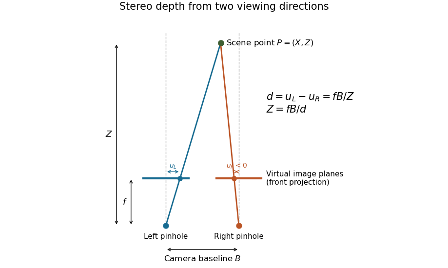
Real cameras require calibration before these simplified equations apply. Stereo rectification transforms the images to an aligned geometry. With noisy measurements, viewing rays need not intersect exactly; minimizing reprojection error instead seeks a point whose projected positions agree as closely as possible with the observations. Reconstruction also depends on stereo correspondence: a mathematically precise intersection of mismatched viewing directions can still describe the wrong scene point.^[ref]

The camera baseline is the separation between the camera centers of two views. For centers $C_L,C_R$, its length is $B=\Vert C_R-C_L\Vert$. It measures translation, so turning a stationary camera without moving its camera center does not create a nonzero camera baseline. A known camera baseline supplies the length scale in stereoscopic triangulation.^[ref]

In the ideal aligned model with matched coordinate origins, stereo disparity satisfies $d=fB/Z$. For focal length 800 pixels and depth 5 metres, a camera baseline 0.10 metres gives 16 pixels; doubling the camera baseline gives 32 pixels. With unchanged disparity precision, the larger separation improves depth sensitivity. It can also increase occlusion in stereo vision and reduce overlap of the views. Finally, multiplying both $B$ and all reconstructed lengths by the same factor leaves the projections unchanged: a small reprojection error alone cannot certify the metric scale.

Stereo rectification transforms a pair of images so that corresponding epipolar lines become aligned scan lines. In a horizontal stereo arrangement, a scene point visible in both rectified views should have the same vertical image coordinate. This turns a two-dimensional matching search into a one-dimensional search along a row.^[ref]

For example, a feature initially at left row 100 and right row 104 can be mapped to the same row in virtual aligned views. Camera calibration supplies geometry for the transforms, and image resampling evaluates the transformed images on a new pixel grid. The new images need not retain every border region. Stereo rectification aligns the geometric search; it does not identify the correct partner among repeated patterns or restore a feature hidden in one view. The rectified focal length and coordinate offsets must also be used when converting stereo disparity to depth.

Stereo correspondence identifies image positions in two views that depict the same scene point. This is the matching step needed before stereoscopic triangulation can recover that point. Epipolar geometry restricts a candidate match to an epipolar line; after horizontal stereo rectification, that search follows a corresponding image row.^[ref]

For example, matching a corner at horizontal coordinate 120 in the left view with coordinate 96 in the right gives stereo disparity 24 pixels. A repeated window pattern might offer equally plausible candidates at 96 and 72, producing different inferred depths. Geometry alone does not choose the correct window. A foreground object can also hide the feature in one view: occlusion in stereo vision then prevents a visible match. Texture, agreement of nearby matches and explicit rejection of ambiguous locations supply evidence beyond mere proximity along a row. A confident disparity map must represent locations where stereo correspondence failed as well as those where it succeeded.

Epipolar geometry describes the projective relationship between two camera views. A scene point away from the camera baseline and the two camera centers determine an epipolar plane. Its intersections with the image planes are corresponding epipolar lines. Knowing one image point therefore constrains its partner to a line rather than the whole second image.^[ref]

With image points in homogeneous coordinates, a fundamental matrix $F$ expresses the constraintFor an ideal horizontally rectified pair this reduces to equality of image-row coordinates, while horizontal displacement remains free and carries stereo disparity. A line constraint does not determine depth: many scene points along one viewing ray satisfy the geometry. Correct stereo correspondence selects a partner, and camera calibration then supports metric stereoscopic triangulation.

Allylic strain is an unfavourable steric interaction involving substituents around the region next to a carbon–carbon double bond. The double bond restricts rotation and makes the relative placement of nearby groups particularly important.

A rotation around an adjacent single bond can reduce crowding while changing which face of the alkene is exposed to a reagent. This provides a route from conformational preference to reaction stereoselectivity. The term should specify the interacting groups and conformation; it is not a universal fixed energy penalty for every allylic fragment.

Tunnel magnetoresistance is the change in resistance of a magnetic tunnel junction when the relative magnetizations of its two electrodes change. A common convention iswhere P and AP denote parallel and antiparallel alignment. This connects quantum tunnelling to the spin dependence of electronic states in the electrodes.

In the Jullière model, assume spin-conserving tunnelling with spin-independent matrix factors, and let the density of states polarizations at the Fermi energy be $P_i=(n_{i\uparrow }-n_{i\downarrow })/(n_{i\uparrow }+n_{i\downarrow })$. Parallel alignment pairs matching spin channels, while antiparallel alignment pairs opposite channels. Hence $G_{\mathrm{P}}\propto 1+P_1{P}_2$ and $G_{\mathrm{AP}}\propto 1-P_1{P}_2$. Using $R=1/G$ givesThis is a consequence of the stated two-channel model, rather than a universal material law.

M. Jullière's 1975 experiment compared the conductance of iron–germanium–cobalt thin-film junctions with parallel and antiparallel magnetizations at low temperature. The thin separating layer, magnetic preparation of the films and conductance measurement together made relative magnetic orientation an experimentally controllable transport variable.^[ref]

The transition frequency between two stationary energy levels is the positive frequency satisfying $h\nu =|E_f-E_i|$. In absorption, the system gains this energy from the radiation; in emission, it loses it. The corresponding angular frequency is $\omega =2\pi \nu$.

An energy difference specifies where a spectral line can occur, but does not by itself guarantee that the transition is strong or allowed. The interaction and its selection rules determine the transition amplitude. External fields, motion and finite lifetimes can shift or broaden the measured line.