For the $110\mathrm{Hz}$ fundamental alone, the Nyquist–Shannon sampling theorem places the limiting sampling rate at twice that frequency:Use a rate strictly above this boundary for a sinusoid of unknown phase: exactly two samples per cycle can, for a particular phase, all fall at zero. If higher Fourier harmonics are retained, the sampling rate must instead exceed twice the highest retained frequency, or those components must be removed to prevent aliasing.

For a straightforward discrete Fourier transform estimate, Fourier frequency resolution obeys $\Delta f\sim 1/T_{\mathrm{obs}}$. Resolving $0.07\mathrm{Hz}$ therefore suggestsAt the limiting sampling rate this is about $f_s{T}_{\mathrm{obs}}\simeq 3143$ samples. These are the usual sampling and spectral-resolution estimates. The $14.3\mathrm{s}$ value is not a universal lower bound on single-tone frequency estimation: fitting a sinusoidal model with sufficiently low noise can estimate its frequency more precisely than the spacing of discrete Fourier transform bins. The question gives no noise level or estimator, so a sharper universal minimum time cannot be deduced.

Let $M$ denote an incident muon and $S$ a detector signal. The selected sample is conditioned on $S$. The law of total probability givesBy Bayes' theorem, the contamination, namely the conditional probability that a selected particle is not a muon, isFor example, per $10000$ incident particles the expected selected counts are $8550$ true muons and $100$ other particles. The denominator is the $8650$ selected particles; the rejected muons are outside this sample.

The Born rule uses the squared modulus of the wavefunction, not its real part. Write $\psi =A[\sin x+i(1-\cos x)]$. ThenWavefunction normalization requiresIntegrating the probability density over the required interval gives the dimensionless probabilityThus approximately $9.08\%$ of position measurements fall in this interval.

The protons at the Large Hadron Collider are ultrarelativistic: their energy is much greater than their rest energy, about $0.938\mathrm{GeV}$. The relativistic energy-momentum relation therefore gives $pc\simeq E$. Using the de Broglie wavelength,Thus the conventional de Broglie wavelength estimate is a distance of order $10^{-19}\mathrm{m}$.

There is a conventional factor of $2\pi$ in interpreting this estimate. Spatial resolution from momentum transfer is often expressed as $\ell \sim \hslash c/Q$, where $Q$ is the transferred momentum multiplied by the speed of light. Taking $Q$ of order the beam energy givesBoth conventions describe the same characteristic scale up to $2\pi$. The beam energy alone does not give an exact experimental spatial resolution: a particular collision probes a scale set by its actual momentum transfer.

Let the infinite outer walls be at $x=0,D$, the finite steps at $x=a,b$, and the three potential energy values be $V_L,V_B,V_R$. The original drawing specifies the orderingThe energy eigenstates can be chosen real. The Dirichlet boundary conditions are $\psi (0)=\psi (D)=0$; wavefunction matching at a finite potential step requires both $\psi$ and ${\psi }^{\prime }$ to be continuous at $a,b$. In particular, neither finite step acts as an additional hard wall.

The time-independent Schrödinger equation givesThus a wavefunction is sinusoidal in a classically allowed region, with wavenumber $k=\sqrt{2m(E-V)}/\hslash$, and a linear combination of exponential functions in a classically forbidden region, with inverse decay length $q=\sqrt{2m(V-E)}/\hslash$. Its curvature changes sign relative to $\psi$ at a step crossing $E$; its slope does not jump.

By the Sturm oscillation theorem, the three energy eigenstates have exactly zero, one, and two interior nodes, respectively. Choose their global phases so that their slopes at the left wall are positive:

For $E_0,E_1$, the right-hand piece is proportional to $\sinh [q_R(D-x)]$, rather than a pure decaying exponential: this enforces the finite-distance hard wall exactly. The barrier pieces likewise contain both exponential solutions. Their small tails are an instance of quantum tunnelling.

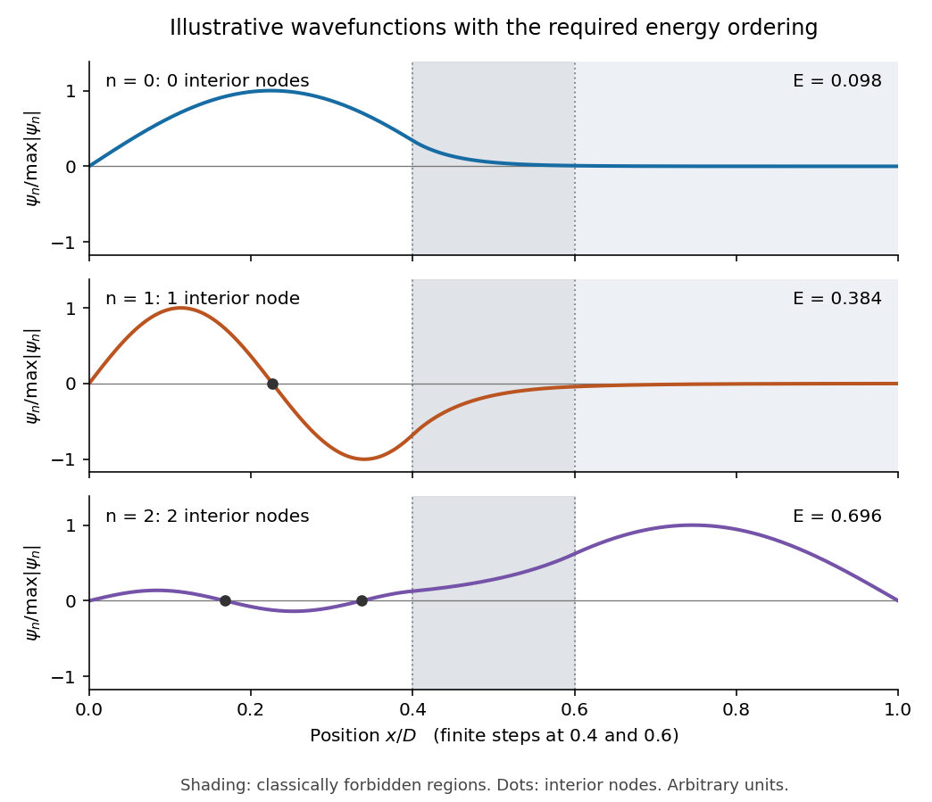
This is an original illustrative calculation, with vertical lines marking only the region boundaries. It uses $D=1$, $a=0.4$, $b=0.6$, $V_L=0$, $V_R=0.62$, $V_B=0.82$, and ${\hslash }^2/(2m{D}^2)=0.002$ in arbitrary energy units. Its lowest energy eigenvalues are approximately $0.098,0.384,0.696$, so it has exactly the required ordering. Here both nodes of the third wavefunction happen to lie towards the left; its dominant lobe is on the right. These precise positions and relative amplitudes are illustrative: the original drawing supplies no numerical lengths, barrier heights, or mass, so it does not determine a unique quantitative wavefunction. The required sketch features are the matching, curvature, hard-wall zeros, and ordered node counts.