Since $A>0$ and $\omega >0$ are fixed, the standard sine limit givesIf $p>-1$, this tends to the assigned value zero. At $p=-1$, the right and left limits are $+A\omega$ and $-A\omega$; if $p<-1$, they diverge with opposite signs. HenceThe cancellation comes from the simple zero of $\sin (\omega x)$ at the origin, not rapid oscillation there.

Among the two orthogonal matrices from part (d)(i), $d=-1$ gives $L=-I$, a rotation matrix through angle $\pi$. For $d=1$, the determinant is $-1$, so the matrix reverses orientation and is a reflection rather than a rotation:It is the reflection matrix across the $y$ axis.

An orthogonal matrix has orthonormal columns. The first column of $L$ has squared norm $1+c^2$, so $c=0$. Orthogonality of the two columns then gives $-b+cd=-b=0$, hence $b=0$. The second column must have squared norm $d^2=1$. ThereforeBoth resulting matrices satisfy $L^{T}L=I$ directly.

For the choice of $B$ in part (b)(i), the two-by-two matrix inverse formula givesMultiplication gives $B{B}^{-1}=B^{-1}B=I$, providing a direct check.

The characteristic polynomial of $A$ isIts distinct eigenvalues are $3$ and $-3$. For $3$, the eigenvector relation gives $y=-2x$, so choose $(1,-2{)}^T$. For $-3$, it gives $x=-2y$, so choose $(2,-1{)}^T$. Put these independent eigenvectors into columns:Then $AB=BC$ column by column. Also $\det B=3\ne 0$, so this choice supplies the diagonalization of a matrix $B^{-1}AB=C$. Scaling columns or interchanging their order gives other valid choices, with the matching order in $C$.

Expanding the determinant along the first row givesUnder the matrix trace condition $a^2=3$, this simplifies to $\det M=b(3-b)$. A square matrix is invertible exactly when its determinant is nonzero. Thus

The matrix trace is the sum of diagonal entries:ConsequentlyThe first diagonal entry is $a^2$ in the original PDF.

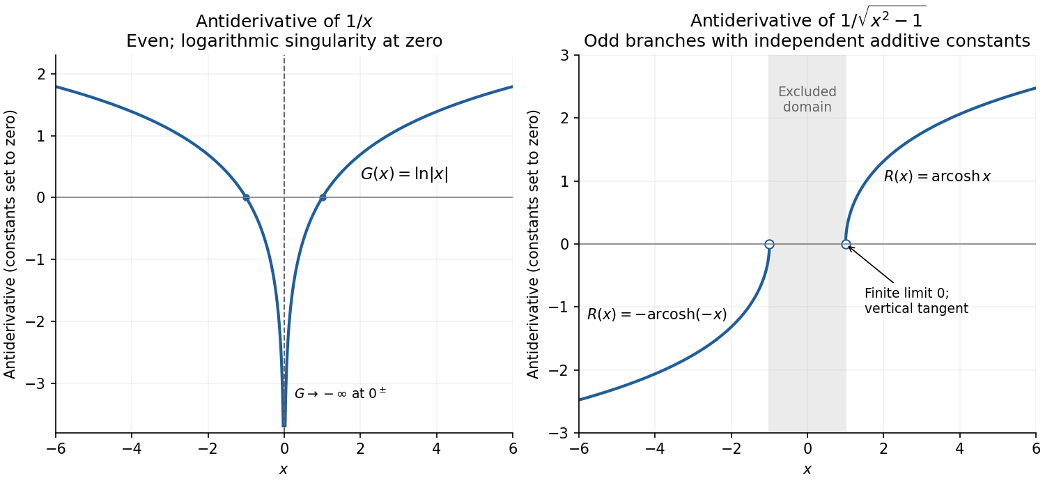
A single formula valid on both real components isLet $s=\sqrt{x^2-1}>0$. Since $x+s\ne 0$,Equivalently, $R(x)=\mathrm{arcosh}x$ for $x>1$ and $R(x)=-\mathrm{arcosh}(-x)$ for $x<-1$. The graph is odd for this choice of constants, increases on both components, and approaches zero with vertical tangent as $x\to 1^{+}$ or $x\to -1^{-}$. Its far-field behaviors are $R(x)\sim \ln (2x)$ on the right and $R(x)\sim -\ln (-2x)$ on the left. The interval $[-1,1]$ is excluded. Independent additive constants could again be assigned to the two components. The right panel sketches these real inverse-hyperbolic antiderivative branches.

At $u=1$, the integrand is unbounded but integrable: $1/\sqrt{u^2-1}\sim [2(u-1){]}^{-1/2}$. Thus the lower-limit integral is understood as an improper integral. With $z=u+\sqrt{u^2-1}$,The lower endpoint corresponds to $z=1$, givingThe limiting value at $x\downarrow 1$ is zero. Here $\mathrm{arcosh}$ is the inverse hyperbolic cosine.

A suitable real antiderivative on the disconnected domain isFor $x>0$, $G^{\prime }=1/x$ directly; for $x<0$, $G=\ln (-x)$ and the chain rule again gives $G^{\prime }=1/x$. The graph is even, crosses zero at $x=\pm 1$, tends to $-\infty$ on either side of zero, and tends to $+\infty$ as $|x|\to \infty$. Independent additive constants may be chosen on the two disconnected half-lines; both are set to zero here.

On the negative half-line, differentiation gives $d\ln (-u)/du=1/u$. The integration path from $-1$ to $x<0$ stays away from the singularity at zero. ThereforeThis choice satisfies $F(-1)=0$.

The sample space outcomes with qualifying sums have totals three, four and five. Their ordered patterns are $(1,1,1)$, the three permutations of $(1,1,2)$, and the three permutations each of $(1,1,3)$ and $(1,2,2)$. Thus there are $1+3+3+3=10$ qualifying outcomes:

To find the probability of exactly one pair, choose its repeated face in six ways, the distinct face in five ways, and which of the three dice has that distinct face in three ways. HenceAs a check, the disjoint events $S,D,T$ exhaust the sample space, and $1/36+5/9+5/12=1$.

Choose the first face in six ways, the second in five ways avoiding the first, and the third in four ways avoiding both. ThusEach ordered outcome is equally likely in this sample space, so dividing the count by $216$ gives the probability.

The sample space has $6^3=216$ equally likely ordered outcomes. The repeated value can be any of the six faces, giving six outcomes $(j,j,j)$. Therefore

Set $dF=0$ in the relative total differential and use the two equal $1\%$ mass increases:Thus the separation must increase by $1\%$. In this special case the result is also exact: the mass product increases by $1.01^2$, and preserving the inverse-square force requires $r_{\mathrm{new}}^2=1.01^2{r}^2$, hence $r_{\mathrm{new}}=1.01r$.

For the force magnitude in Newton's law of universal gravitation, the total differential isDividing by the positive value $F$ gives the particularly useful relative formFor finite small changes this gives the first-order approximation to the fractional change; higher-order products of increments are omitted.

Combine the complementary function and particular solution:The boundary condition at zero gives $C_1+2/3=0$, while that at $\pi /2$ gives $C_2+1/3=0$. HenceThe two boundary conditions determine both constants uniquely; substitution at each endpoint gives zero.

Use the method of undetermined coefficients, choosing a particular solution $y_p=A+B\cos 2x$. Substitution givesMatching the constant and cosine coefficients to $\frac{1}{2}-\frac{1}{2}\cos 2x$ gives $A=1/2$, $B=1/6$. ThusNeither forcing term is resonant with the homogeneous angular frequency one.

The homogeneous linear differential equation is $y^{\prime \prime }+y=0$. Its characteristic equation is ${\lambda }^2+1=0$, with roots $\pm i$. The general real complementary function is thereforeThe two trigonometric solutions are linearly independent, supplying the two arbitrary constants required for this second-order linear ordinary differential equation.