Put $d=\sqrt{a^2-b^2-c^2}>0$ and $h=b-ic$. The denominator of the complex rational function becomesThe quadratic formula gives its two zeros, hence the two poles:Their product is $(b+ic)/(b-ic)$, so $|z_{\mathrm{in}}{z}_{\mathrm{out}}|=1$. To locate them one also needs to exclude the possibility of both lying on the unit circle. Here their moduli are explicit:Both are simple poles: $P^{\prime }(z)=hz+a$ takes the nonzero values $d$ and $-d$ at them. In particular their residues are $1/d$ and $-1/d$.

For the real integral, use the change of variables $z=e^{i\theta }$. As $\theta$ runs from $-\pi$ to $\pi$, this traverses the unit circle once counterclockwise, andThus $I=(1/i){\oint }_{|z|=1}f(z)dz$. Only $z_{\mathrm{in}}$ is enclosed. The residue theorem, or Cauchy integral formula after subtracting its simple-pole part, givesThe real denominator is positive because $a>\sqrt{b^2+c^2}$. As an independent check, write $b\cos \theta +c\sin \theta =\sqrt{b^2+c^2}\cos (\theta -\varphi )$; a period shift reduces the answer to the existing reciprocal affine sine integral.

The outgoing Green function for the three-dimensional Helmholtz equation satisfiesIts normalization follows by integrating over a small ball about $x$: $G_F\sim 1/(4\pi |y-x|)$, so its outward derivative has flux $-1$. Apply Green's second identity in the $y$ variables:The ${\omega }^2$ terms cancel. Thus the surface integral equals $-\Psi (x)$ for $x\in V$, and zero for $x$ outside the closed volume. Equivalently, remove a small source ball and evaluate its flux before taking its radius to zero. A source on the boundary would require a different limiting formula and is not part of this calculation.

For the upper half-space, take a half-ball of radius $\rho$. Interpret the first far-field condition as $\Psi =O({\rho }^{-1})$, and the radiation limit in its usual direction-uniform sense, namely the Sommerfeld radiation conditionThis is the finite-bound interpretation of the PDF's first condition. For fixed $x$ and real $\omega$,Indeed $|y-x|=\rho -\hat{y}\cdot x+O({\rho }^{-1})$, and its radial derivative is $1+O({\rho }^{-2})$. On the large hemisphere the integrand can therefore be rewritten asIts area is $2\pi {\rho }^2$, so its integral tends to zero. The planar integral, taken over expanding disks if needed, consequently equals $-\Psi (x)$ for $x_3>0$ and zero for $x_3<0$.

The outward unit normal vector on the bottom plane is $-e_3$. Denote this planar integral byFor $x_3>0$ reflect the source point to $x^{\ast }=(x_1,x_2,-x_3)$. On the plane,Adding $I(x)=-\Psi (x)$ and $I(x^{\ast })=0$ cancels the boundary values of $\Psi$ and gives $2\int G_F{\partial }_3\Psi =-\Psi (x)$. Thus the Neumann representation for a radiating Helmholtz half-space isThe negative sign is consistent with using the upward derivative ${\partial }_3\Psi$ rather than the outward normal derivative. If that upward derivative is zero everywhere on the plane, the integral is zero. Hence $\Psi =0$ throughout the upper half-space in the specified radiating class; taking a difference also gives uniqueness for prescribed Neumann boundary data.

Use separation of variables, $\Phi =F(r)H(\theta )$, in the Laplace equation in polar coordinates. Dividing by $FH/r^2$ givesSingle-valued $2\pi$-periodic angular factors have integer $n\ge 0$. For $n\ge 1$, they are $\cos n\theta ,\sin n\theta$, and the radial equation $r^2{F}^{\prime \prime }+r{F}^{\prime }-n^{2}F=0$ has solutions $r^n,r^{-n}$. The zero angular mode gives $F=a_0+b_0\log r$. These separated products give the requested solutions; arbitrary sums may use independent coefficients for each radial-angular combination.

Boundedness at the origin removes the logarithm and all negative radial powers. The boundary function is even, so its sine Fourier coefficients vanish. With the convention $f(\theta )=a_0+{\sum }_{n\ge 1}{a}_n\cos n\theta$, its Fourier coefficients areThus the bounded interior harmonic extension isFor $r<R$ the series and its derivatives converge locally uniformly, so it is harmonic. It is a rotated and scaled instance of the harmonic measure of a semicircle in a disk. For example, summing the power series for the complex arctangent, or differentiating the following expression, gives the equivalent real formThis also proves boundedness directly.

At the two jumps, the boundary interpretation matters. At every continuity point the radial limit equals the prescribed value. At $\theta =\pm \pi /2$, the radial limit is $C/2$, the midpoint of the two one-sided values. Consequently for $C\ne 0$ there is no harmonic solution continuous on the closed disk with exactly the printed boundary values. The standard bounded Dirichlet problem imposes the trace away from the jumps, or almost everywhere; assigning zero separately at those two boundary points does not alter the interior solution.

For uniqueness let $w=\tilde{\Phi }-\Phi$. Formally the divergence theorem applied to $w\nabla w$ givesFor continuous zero boundary data, this immediately forces $w=0$. With the actual discontinuous data, one should justify the two exceptional points rather than assume finite Dirichlet energy there. Let $|w|\le M$ and choose a cutoff ${\eta }_{ϵ}$ which is zero within ${ϵ}^2$ of those points, one beyond $ϵ$, and linear in logarithmic distance between. Its gradient satisfies $\int |\nabla {\eta }_{ϵ}{|}^2=O(1/|\log ϵ|)$. Applying the divergence theorem to ${\eta }_{ϵ}^{2}w\nabla w$ givesThe resulting energy tends to zero. Hence $\nabla w=0$ on every compact subset and $w$ is constant; its zero boundary trace on the open arcs makes it zero. This is the logarithmic cutoff proof of harmonic uniqueness with finitely many boundary exceptions.

For the exterior harmonic extension of disk boundary data, boundedness instead excludes $r^n$ and the logarithm. The same boundary coefficients giveThis is ${\Phi }_{\mathrm{in}}(R^2/r,\theta )$, using inversion in a circle. Its limit at infinity is $C/2$. To see why that value is forced independently of this construction, average any bounded exterior harmonic function over a circle. The mean satisfies $(r{\overline{\Phi }}^{\prime }{)}^{\prime }=0$, hence is $A+B\log r$. Boundedness forces $B=0$, and the boundary mean fixes $A=C/2$. A constant limit at infinity must therefore be $C/2$.

Finally suppose two bounded exterior solutions have this limit. Their difference $w$ tends to zero. Under planar inversion in a circle, it is bounded and harmonic near the origin, so the isolated point there is removable. Its local expansion gives $w=O(r^{-1})$, ${\partial }_{r}w=O(r^{-2})$ in the original exterior. Apply the preceding divergence theorem energy argument on $R<r<L$, with logarithmic cutoffs at the two boundary jumps. After removing those cutoffs, the inner boundary term vanishes; the outer one is ${\int }_{r=L}w{\partial }_{r}wds=O(L^{-2})$. Letting $L\to \infty$ forces $\nabla w=0$, and the zero limit gives $w=0$. Thus the bounded exterior solution is unique as well.

A group representation on a vector space $W$ is a group homomorphism $\rho :G\to GL(W)$: $\rho (gh)=\rho (g)\rho (h)$ and $\rho (e)=I$. An invariant subspace $U$ obeys $\rho (g)U\subseteq U$ for every $g$. A nonzero representation is irreducible if its only invariant subspaces are $0$ and $W$. It is a faithful representation if it is injective, equivalently if its group kernel is $\{e\}$. Its character is ${\chi }_{\rho }(g)=\mathrm{tr}\rho (g)$. For inequivalent complex irreducible representations of a finite group, character orthogonality is

Use right-to-left composition of permutations and assign the matrix labels consistently byThe resulting Cayley table, with row multiplying column, isConjugation relabels the entries of a cycle, preserving its length. Thus the conjugacy classes are

Define the permutation representation by $P_{\sigma }{e}_j=e_{\sigma (j)}$, or $(P_{\sigma }{)}_{ij}={\delta }_{i,\sigma (j)}$. Applying it to a basis vector proves $P_{\sigma }{P}_{\tau }=P_{\sigma \tau }$. The six assignments above produce exactly the listed matrices. They are distinct, and $P_{\sigma }=I$ forces $\sigma (j)=j$ for every $j$, so the representation is faithful.

Every permutation fixes $(1,1,1)$, hence fixes every vector $(c,c,c)$. Therefore $V_0$ is a one-dimensional invariant subspace carrying the trivial representation. Its orthogonal complement issince the inner product with $(c,c,c)$ is $c(v_1+v_2+v_3)$. Permuting coordinates preserves their sum, so this plane is invariant too. Every real vector has the unique decompositionThus the permutation representation is the direct sum of group representations on the line and the plane.

To find the eigenvectors of $A$, note that $A(v_1,v_2,v_3)=(v_3,v_1,v_2)$. With $\zeta =e^{2\pi i/3}$, its three eigenvalues and eigenspaces areThe only real eigenvalue is one, whose eigenline is $V_0$, so $A$ has no nonzero real eigenvector in $V_0^{\perp }$. A proper nonzero real invariant subspace of that two-dimensional plane would be a line, giving such an eigenvector. Hence the plane representation is irreducible over $\mathbb{R}$.

For the later complex dimension-count theorem one should also establish irreducibility over $\mathbb{C}$; real irreducibility alone would not imply it in general. In the complexified plane, the only candidate $A$-invariant lines are its $\zeta$ and ${\zeta }^2$ eigenlines. But $C$ exchanges them:Neither is invariant under the whole group, proving complex irreducibility as well. The required decomposition is thereforewhere $W$ is the standard representation of the symmetric group for three letters. Its character is obtained by subtracting one from the number of fixed coordinates: on the three classes it is $(2,-1,0)$.

Finally, the sign representation gives a second one-dimensional irreducible, with value $+1$ on $I,A,B$ and $-1$ on the transpositions. These are exactly the two one-dimensional possibilities: if $r=A,s=C$, a one-dimensional representation sends them to commuting nonzero scalars $v,u$. The relations $r^3=s^2=e$ and $srs=r^{-1}$ imply $v^3=u^2=1$ and $v=v^{-1}$. Hence $v=1$ and $u=\pm 1$, the trivial and sign choices. Together with the two-dimensional $W$, these giveThe sum of squares of irreducible representation dimensions leaves room for no other irreducible. Thus there are exactly two one-dimensional and one two-dimensional complex irreducible representations.

For fixed endpoint values, the Euler-Lagrange equation is $f_y-d{f}_{y^{\prime }}/dx=0$. Along a stationary curve, the chain rule givesWhen $f_x=0$, the Beltrami identity therefore takes the requested sign convention

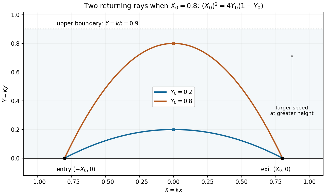
By Fermat principle, the elapsed-time integrand for the given speed is $f=c_0^{-1}\sqrt{1-ky}\sqrt{1+(y^{\prime }{)}^2}$. ThusThe constant is negative for a finite regular ray. Squaring gives $(1-ky)/(1+(y^{\prime }{)}^2)=c_0^2{A}^2$. At a maximum height $y_0$, the slope is zero, so $c_0^2{A}^2=1-k{y}_0>0$. HenceSeparate variables on either side of the turning point. Integration gives the parabolic light rays in a reciprocal-square-root speed profileThe quadratic opens downwards, with its greatest height $y_0$ at $x=x_c$. The positive index condition holds throughout the layer because $kh<1$. Vertical rays are a separate zero-horizontal-momentum case, outside the regular graph representation $y(x)$; they are not returning rays of the type considered below.

Equal endpoint heights at $x=\pm x_0$ force $x_c=0$. Setting $y(\pm x_0)=0$ givesFor nonzero separation, a real returning ray requires $k{x}_0\le 1$ and has candidate turning heightsOnly choices satisfying $0<y_0<h$ are rays wholly within the specified layer. Depending on its thickness there may be two, one, or no admissible choices; at zero discriminant the two algebraic candidates coincide. The entry and exit points at $y=0$ are interpreted as limiting boundary points of the open medium.

In monic form the Chebyshev differential equation has $P(x)=-x/(1-x^2)$ and $Q(x)=p^2/(1-x^2)$. Both are analytic near zero, so it is an ordinary point. At $x=1$, $(x-1)P=x/(x+1)$ and $(x-1{)}^{2}Q=-p^2(x-1)/(x+1)$ are analytic; at $x=-1$, $(x+1)P=x/(x-1)$ and $(x+1{)}^{2}Q=-p^2(x+1)/(x-1)$ are analytic. Thus both endpoints are regular singular points.

Insert $y_q={\sum }_{n\ge 0}{a}_n{x}^{n+q}$ and equate coefficients. The recurrence relation isExplicitly the factors are $(n^2-p^2)/[(n+2)(n+1)]$ for $q=0$ and $[(n+1{)}^2-p^2]/[(n+3)(n+2)]$ for $q=1$. The lowest equation for $q=1$ forces $a_1=0$. For $q=0$, one may choose $a_1=0$ to select an even solution, independent of the odd $q=1$ solution. The leading coefficient $a_0$ is free in either chosen parity branch.

For a nonterminating branch the consecutive parity-term ratio tends to $x^2$. Hence the ratio test gives convergence for $|x|<1$, and radius of convergence one. Terminating branches are polynomials with infinite radius. For $p=m\ge 0$ an integer, choose $q$ of the same parity as $m$: the recurrence stops once $n+q=m$, producing a degree-$m$ Chebyshev polynomial. Normalization at $1$ gives all nonzero coefficients through degree three:

Set $Y(\theta )=y(\cos \theta )$. Direct differentiation gives $Y^{\prime \prime }={\sin }^2\theta y^{\prime \prime }-\cos \theta y^{\prime }$, so the equation becomes $Y^{\prime \prime }+m^{2}Y=0$. For $m>0$, $Y=A\cos (m\theta )+B\sin (m\theta )$. A polynomial $y$ has finite derivative at $x=1$, and therefore $Y^{\prime }(0)=-\sin 0y^{\prime }(1)=0$, forcing $B=0$. Also $Y(0)=T_m(1)=1$, so $A=1$. For $m=0$, the transformed solution is affine in $\theta$ and the same derivative condition removes its linear term. ThusThe endpoint values follow by continuity. The finite-derivative condition is what excludes the independent nonpolynomial branch, rather than normalization alone.

Evaluate the derivative along real and imaginary increments. For a holomorphic function, both give the same value:Equating real and imaginary parts yields the Cauchy-Riemann equations