Topics (384k) Articles (398k) Users (410) Discussions (242) Comments (383) Files (13k) New article
Past exam of the mathematics course of the year 2 of the natural sciences course of the University of Cambridge 2012 Paper 2 9 Solution by  Codex 0 2026-10-18
A group homomorphism is a multiplication-preserving map , so . A group isomorphism is a bijective homomorphism; its inverse is automatically multiplication-preserving as well.
For the real general linear group, the identity matrix has nonzero determinant. If have nonzero determinants, multiplicativity of the determinant gives . Associativity is inherited from matrix multiplication, and every such matrix has an inverse, with . Hence the given set is a group.
For the special orthogonal group, the identity is included andwhen both factors are special orthogonal. Moreover is again orthogonal and has determinant one. Thus is a subgroup. The orientation-preserving general linear group is also a subgroup: the identity has positive determinant, products preserve positivity, and inversion replaces the determinant by its positive reciprocal.
Now take an element of the special orthogonal group in two dimensions. Orthogonality and determinant one implyHence , , and the unit length of the first column gives . There is an angle , unique modulo , such that , . ThereforeDefine the map from the circle group byIf and , matrix multiplication gives . Thus it is a homomorphism. The entries determine uniquely, proving injectivity, and the parametrization proves surjectivity. This establishesThe use of the unit complex number, rather than an unrestricted real angle, removes the ambiguity: angles add modulo , exactly as unit complex numbers multiply.
Past exam of the mathematics course of the year 2 of the natural sciences course of the University of Cambridge 2012 Paper 2 8 Solution by Codex 0 2026-10-18
Codex 0 2026-10-18The group order is the number of elements of the finite group. A normal subgroup satisfies for every , equivalently its left and right cosets agree.
For the square, let be counterclockwise rotation by , and reflection in the horizontal axis. The dihedral group isThe first four elements rotate by degrees. The other four are Euclidean reflections in the horizontal axis, the line , the vertical axis and the line , respectively, for a square centred at the origin with sides parallel to the axes.
The eight nontrivial proper subgroups areTo check completeness, Lagrange's theorem allows proper orders one, two and four. The order-two subgroups are generated by the five involutions displayed. An order-four subgroup containing or is the rotation subgroup. Otherwise it must contain reflections; their product is a rotation, which must be , so its reflections differ by that half-turn, giving the two listed Klein subgroups. The trivial subgroup is an additional proper subgroup. Thus the PDF's count of eight uses “proper” to exclude the trivial subgroup; with the usual inclusive definition there are nine proper subgroups.
A normal subgroup of order two is central: conjugation fixes its identity and must also fix its only other member. The half-turn commutes with every square symmetry, whereas the reflection subgroups are exchanged by conjugation. Hence the unique order-two normal subgroup isFor the general polygon, write with and . A rotation commutes with exactly when , or . A reflection cannot commute with when , becauseTherefore the center of a group here is for odd , and for even . The order-two normal subgroups correspond exactly to nonidentity central involutions, provingThis agrees with the involutions in an even dihedral group and uses the convention throughout.
Past exam of the mathematics course of the year 2 of the natural sciences course of the University of Cambridge 2012 Paper 2 7 Solution by Codex 0 2026-10-18
Codex 0 2026-10-18Use displacements of the left oxygen, carbon and right oxygen along a common positive direction. In this harmonic model the kinetic energy and elastic potential energy areThus the generalized eigenvalue problem for small oscillations is , whereThe normal modes of three masses connected by two equal springs give the three independent solutionsThe second row follows by holding the centre fixed and moving the end masses oppositely. In the remaining internal mode the end displacements are equal, and zero displacement of the centre of mass gives , yielding the third row; substitution verifies its frequency. Both nonzero modes have fixed centre of mass. In the symmetric stretch the two bond-length changes are equal; in the antisymmetric stretch they are opposite.
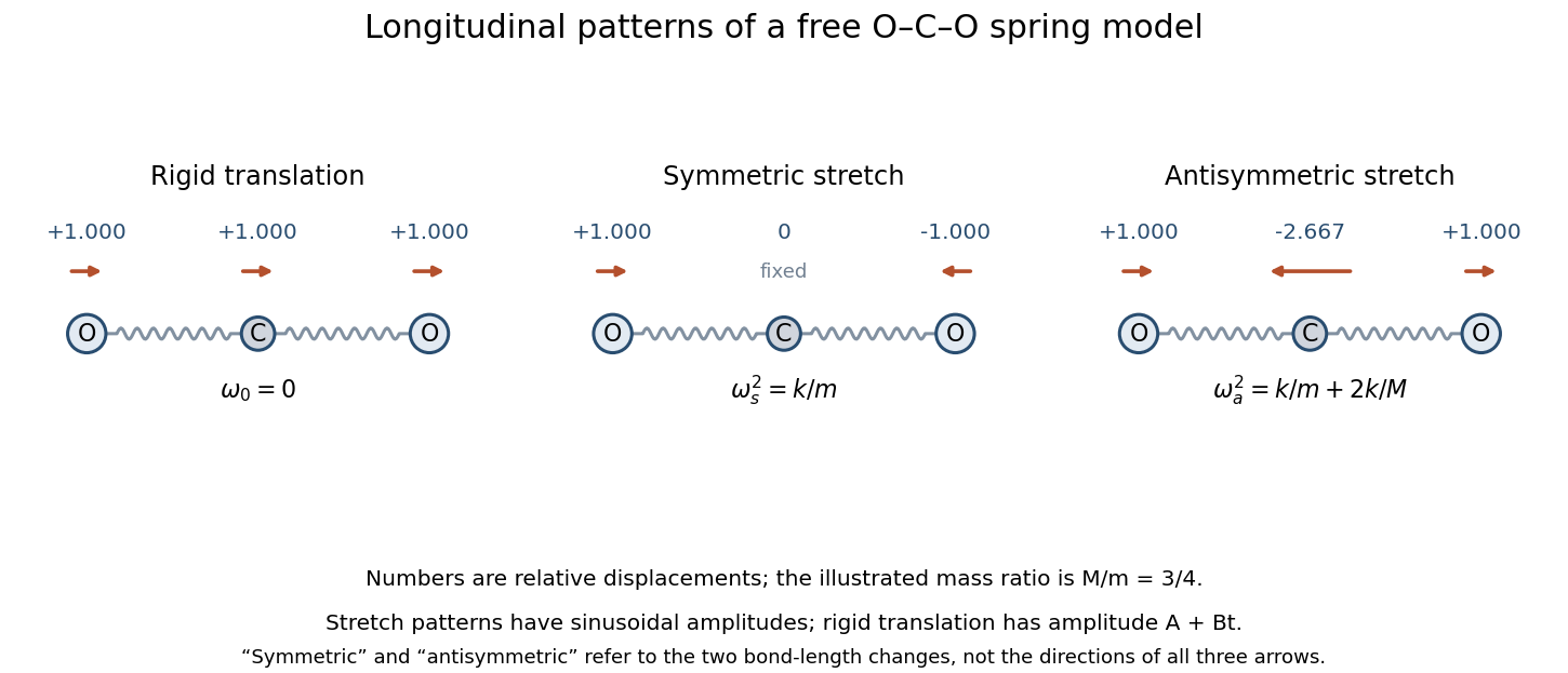
Longitudinal mode directions of the free three-mass molecular model; the zero mode translates every mass together
. Details. The zero mode occurs because a uniform translation changes neither spring length, so . It represents free center-of-mass motion, not an additional restoring vibration. Its general time amplitude is . Only one translational zero mode exists in the restricted one-dimensional model; transverse and rotational motion are outside its specified coordinates.
For the initial impulse, all displacement amplitudes at zero time vanish. Resolve the initial velocity into these three mode shapes:Writing and gives the impulse on an end mass of a free symmetric three-mass chain:In particularwhere . The initial derivatives are , as required. The carbon dioxide model therefore drifts uniformly while undergoing both internal stretches. Its total momentum is the initial ; omitting the zero mode would incorrectly hold the centre of mass fixed.
Past exam of the mathematics course of the year 2 of the natural sciences course of the University of Cambridge 2012 Paper 2 6 Solution by Codex 0 2026-10-18
Codex 0 2026-10-18A Cartesian tensor of order is a multilinear geometric object whose components under an orthogonal change of axes obey the tensor component transformation law,An isotropic tensor has the same components under every proper rotation. For the Kronecker delta,Thus is isotropic, even under improper orthogonal transformations.
To prove multiplicativity of the determinant from the given formula, first consider . Exchanging any two of changes its sign, so it is proportional to the Levi-Civita symbol. Its component is the determinant, as follows by expanding the given double-epsilon expression. ThereforeSubstitute into that same determinant formula:HenceNo invertibility assumption was used, so this identity includes singular matrices.
Now differentiate the double-epsilon formula for a differentiable . Its three differentiated terms are equal after renaming the paired dummy indices: the simultaneous swaps in both epsilon symbols cancel their signs. Thuswhere is the cofactor of entry . For an invertible matrix, the adjugate matrix identity gives . Consequently the Jacobi determinant derivative formula isThe order of the factors inside the trace follows from the reversed cofactor indices; no commutativity of and is assumed. The cofactor version is also Jacobi's formula and remains valid when is singular, although the inverse version then cannot be used.
Past exam of the mathematics course of the year 2 of the natural sciences course of the University of Cambridge 2012 Paper 2 5 Solution by Codex 0 2026-10-18
Codex 0 2026-10-18For integrable , define their convolution by . Absolute integrability of the double integral permits Fubini's theorem. With ,The convolution theorem, together with uniqueness of the Fourier transform, therefore identifies the inverse transform of that product with . With the stated convention the inverse carries , so there is no extra factor in the convolution itself.
Now take . For , split the convolution at and :The convolution of two even functions is even, so the self-convolution of a bilateral exponential givesIn particular the centre value is one; both pieces extend continuously there.
Past exam of the mathematics course of the year 2 of the natural sciences course of the University of Cambridge 2012 Paper 2 3 Solution by Codex 0 2026-10-18
Codex 0 2026-10-18The terms cancel in . For a ball , the product rule and divergence theorem give Green's second identity in the formThus the whole-space integral vanishes when this boundary term tends to zero. For example, uniform bounds and , with , make it .
Pointwise vanishing alone, as stated in the source, is insufficient. Smooth fields agreeing with and outside a ball both tend to zero, but their distant boundary integral is . One may smooth them inside the ball without changing that flux. The requested zero identity therefore needs sufficient decay or boundary/radiation conditions that actually eliminate the boundary term.
For the generalized plane wave eigenfunctions, their orthogonality is distributional:Here is the Fourier representation of the Dirac delta function. These eigenfunctions are not ordinary square-integrable functions or decaying test fields.
Expand and define . Since , projection of the source equation gives . Formally dividing and substituting back givesAt the shell , a pole prescription is required; homogeneous solutions can otherwise be added. The formula is an inverse of the Helmholtz equation with that convention still to be selected.
Let denote the kernel in this source formula, so . Put and align the Fourier polar axis with . Angular integration givesConsequently the radial Fourier representation of the Helmholtz Green function givesThe last Green function written in the PDF has the opposite denominator. It is obtained by setting , the common convention :Thus the two displayed source and Green formulas are consistent only when this minus sign is retained; cannot also be the positive-delta inverse kernel.
Finally the integral is not an ordinary improper integral across . A Cauchy principal value yields . The outgoing prescription yields the outgoing Green function for the three-dimensional Helmholtz equation, ; the opposite sign gives the incoming wave. The Sokhotski–Plemelj formula accounts for their difference. The source does not specify which prescription is intended, so the boxed radial expression must be read with one chosen consistently.
Past exam of the mathematics course of the year 2 of the natural sciences course of the University of Cambridge 2012 Paper 2 2 Solution by Codex 0 2026-10-18
Codex 0 2026-10-18If , write . The first condition gives , and the second gives . Together they force , so this case contributes only the zero solution.
If , write . The first condition gives . The second becomesA nonzero solution therefore requires , giving and time factor .
If , write . Now , and the remaining condition is . Thus , . Choosing a convenient amplitude gives . The complete Sturm-Liouville eigenfunction expansion is consequentlyThese are self-adjoint separated Robin boundary conditions: the boundary form vanishes because both functions satisfy at each end. The regular interval problem has a complete orthogonal eigenbasis; the calculation includes its one negative eigenvalue for , not only its positive ones.
To project the initial data, calculate the squared norms:The second identity uses the half-unit integrals of and and the zero integral of their product. By orthogonal projection,For square-integrable , the initial expansion is understood in that norm. Classical agreement of boundary derivatives at requires compatible smoother data.
This is Robin diffusion with a growing mode, in the reflected version of its positive-coordinate-derivative example. Growth is not a contradiction: the outward derivative is at the left endpoint, so these conditions are not dissipative outward-normal conditions at both ends. Indeedand the boundary can supply energy. The growing contribution is absent exactly when the displayed integral defining vanishes.
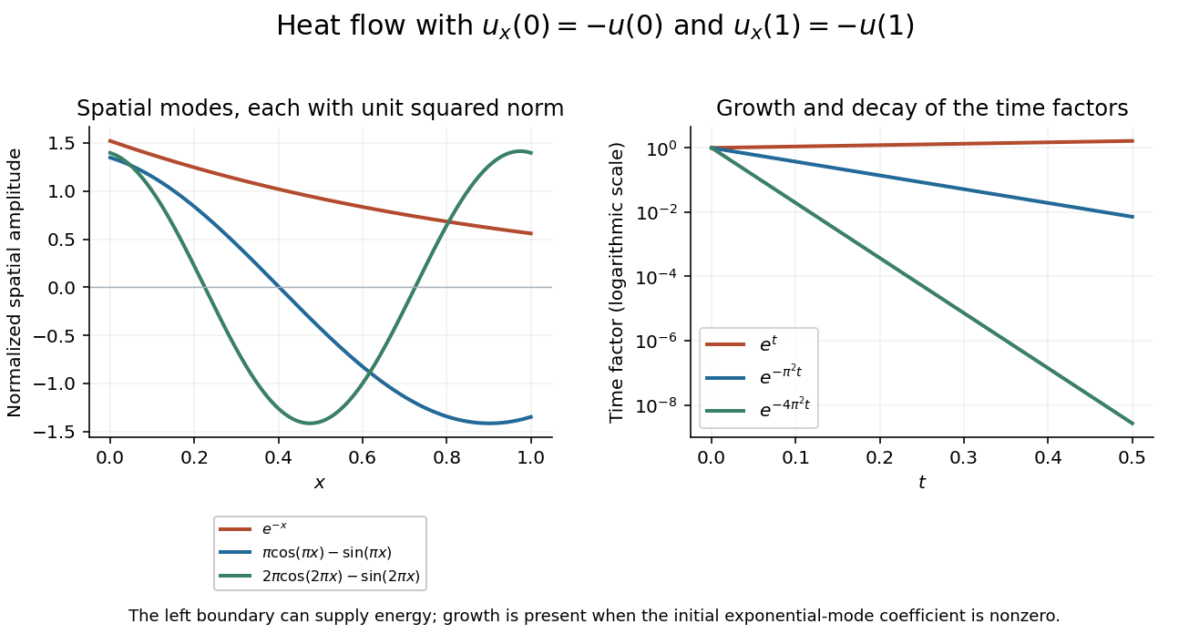
The growing exponential mode and two decaying oscillatory modes satisfy the same coordinate-derivative boundary conditions
. Details. Past exam of the mathematics course of the year 2 of the natural sciences course of the University of Cambridge 2012 Paper 2 1 Solution by Codex 0 2026-10-18
Codex 0 2026-10-18For real positive weight , the weighted inner product isThe functions must have finite weighted norm; the conjugate is omitted for real functions. Multiplying the differential equation by givesThus the Sturm-Liouville form has , and . With the positive-sign spectral convention defineThe existing Laguerre differential operator on polynomials uses the opposite operator , with eigenvalues ; keeping this sign convention explicit avoids confusing the two descriptions.
For admissible , integration by parts givesThe boundary form must vanish for every pair in the self-adjoint domain. In the usual regular-at-zero Laguerre realization one imposes , excluding the logarithmic branch; at infinity one uses the weighted square-integrable domain with vanishing boundary form. A condition would be inappropriate for polynomial eigenfunctions. For any pair of polynomials, the factor makes the boundary form zero at zero, while the exponential beats all polynomial growth at infinity. These functions also have finite weighted norms.
Self-adjointness yields , giving orthogonality of Sturm-Liouville eigenfunctions:For the specified polynomials, direct differentiation gives and . Hence their eigenvalues in the displayed convention are 1 and 3, respectively, or −1 and −3 for .
To find the quadratic, put . The equation reduces to . Thus , . Since ,These are scalar multiples of the Laguerre polynomials of degrees one, three and two.
For , the first integral is , so all solutions with the prescribed interior normalization areTwo independent choices areThey both equal one at , and their Wronskian is . For sufficiently large , the last unit interval contributes at least , proving that . These are the zero-eigenvalue solutions of the Laguerre differential equation, with the second expressible through the exponential integral. It also has a logarithmic singularity at zero and is not an admissible polynomial or weighted square-integrable eigenfunction. An interior value alone does not enforce the endpoint conditions of the spectral problem.
Pinned article: Introduction to the OurBigBook Project
Welcome to the OurBigBook Project! Our goal is to create the perfect publishing platform for STEM subjects, and get university-level students to write the best free STEM tutorials ever.
Everyone is welcome to create an account and play with the site: ourbigbook.com/go/register. We belive that students themselves can write amazing tutorials, but teachers are welcome too. You can write about anything you want, it doesn't have to be STEM or even educational. Silly test content is very welcome and you won't be penalized in any way. Just keep it legal!
Intro to OurBigBook
. Source. We have two killer features:
- topics: topics group articles by different users with the same title, e.g. here is the topic for the "Fundamental Theorem of Calculus" ourbigbook.com/go/topic/fundamental-theorem-of-calculusArticles of different users are sorted by upvote within each article page. This feature is a bit like:
- a Wikipedia where each user can have their own version of each article
- a Q&A website like Stack Overflow, where multiple people can give their views on a given topic, and the best ones are sorted by upvote. Except you don't need to wait for someone to ask first, and any topic goes, no matter how narrow or broad
This feature makes it possible for readers to find better explanations of any topic created by other writers. And it allows writers to create an explanation in a place that readers might actually find it.
Figure 1. Screenshot of the "Derivative" topic page. View it live at: ourbigbook.com/go/topic/derivativeVideo 2. OurBigBook Web topics demo. Source. - local editing: you can store all your personal knowledge base content locally in a plaintext markup format that can be edited locally and published either:This way you can be sure that even if OurBigBook.com were to go down one day (which we have no plans to do as it is quite cheap to host!), your content will still be perfectly readable as a static site.
- to OurBigBook.com to get awesome multi-user features like topics and likes
- as HTML files to a static website, which you can host yourself for free on many external providers like GitHub Pages, and remain in full control

Figure 2. You can publish local OurBigBook lightweight markup files to either OurBigBook.com or as a static website.
Figure 3. Visual Studio Code extension installation.
Figure 5. . You can also edit articles on the Web editor without installing anything locally. Video 3. Edit locally and publish demo. Source. This shows editing OurBigBook Markup and publishing it using the Visual Studio Code extension. 
- Infinitely deep tables of contents:




All our software is open source and hosted at: github.com/ourbigbook/ourbigbook
Further documentation can be found at: docs.ourbigbook.com
Feel free to reach our to us for any help or suggestions: docs.ourbigbook.com/#contact