An eigenvalue $\lambda$ and associated eigenvector $e\ne 0$ satisfy $Ae=\lambda e$. The characteristic polynomial $\det (A-\lambda I)$ has degree equal to the positive matrix size. The fundamental theorem of algebra gives a complex root, at which $A-\lambda I$ is singular and therefore has a nontrivial kernel. Hence every nonempty square complex matrix has an eigenvector.

A nondiagonalizable example is the Jordan block $\left(\begin{array}{cc}0& 1\\ 0& 0\end{array}\right)$: its only eigenvalue is zero, and its eigenspace is one-dimensional. A Hermitian matrix satisfies $A^{†}=A$ and has an orthonormal eigenbasis by the spectral theorem. One proof finds an eigenvector, notes that its orthogonal complement is invariant, and repeats. Its eigenvalues are real becausewhere $e^{†}e>0$.

With all eigenvalues negative, $A$ is invertible. Its same complete eigenbasis givesSome powered eigenvalues can coincide, but the original eigenvectors remain a complete basis. Writing $A=U\mathrm{diag}({\lambda }_i)U^{†}$, the convergent matrix exponential series givesThus the matrix inverse from a decaying matrix exponential isThe identity printed in the original PDF is missing a minus sign. Already for the one-by-one matrix $A=(-1)$ its integral is $1$, whereas its inverse is $-1$. Equivalently, integrating $d(e^{tA})/dt=A{e}^{tA}$ gives $A{\int }_0^{\infty }{e}^{tA}dt=-I$, confirming the correction without diagonalization.

Split the Fourier transform integral at zero:By Fourier inversion applied to this pair, or by the residue theorem, the other transform isFor example, inversion with $\lambda =\mu$ gives $\int e^{ikx}(k^2+{\mu }^2{)}^{-1}dk=(\pi /\mu )e^{-\mu |x|}$; evenness supplies the desired sign convention.

Take the spatial Fourier transform of the Laplace equation. For $y>0$ it gives ${\hat{\psi }}_{yy}-k^2\hat{\psi }=0$. Removing the exponentially growing solution and matching the boundary givesAt $k=0$ this formula is interpreted by continuity; a single transform value does not alter the inverse integral. The previous transform pair identifiesthe Poisson kernel for the upper half-plane. The convolution theorem therefore gives the Poisson integralThis is the bounded harmonic solution for bounded decaying data, or the corresponding solution in an appropriate Fourier class. Such a growth condition matters if vertical decay is interpreted only pointwise: the nonzero harmonic function $e^{x^2-y^2}\sin (2xy)=\mathrm{Im}{e}^{(x+iy{)}^2}$ vanishes on the real axis and tends to zero for fixed $x$ as $y\to \infty$, but grows rapidly in $x$ and has no ordinary spatial Fourier transform. It can be excluded by requiring boundedness; the stated pointwise limits alone would not establish uniqueness.

For the interval data, direct integration gives the Poisson extension of interval boundary dataAs $y\downarrow 0$ it approaches $c$ for $|x|<a$, zero for $|x|>a$, and $c/2$ at $x=\pm a$. At those jump points the prescribed isolated values cannot be attained by a continuous extension; they do not affect the integral. The solution decays vertically, with $\psi \sim 2ac/(\pi y)$ for fixed $x$ and large $y$.

Expand the radial modified Helmholtz equation as $Ly=-y^{\prime \prime }-2y^{\prime }/x+y$. Setting $y=z/x$ gives $Ly=(-z^{\prime \prime }+z)/x$, soBoundedness at zero requires $A+B=0$, whereas boundedness at infinity requires $A=0$. The respective adapted homogeneous solutions are thereforeThe first has limit one at zero. Their Wronskian is $u{v}^{\prime }-u^{\prime }v=-x^{-2}$. Since the highest-derivative coefficient of $L$ is $-1$, the Green function must have first-derivative jump $-1$. The radial modified Helmholtz Green function on the half-line isIt is continuous at the source, and its derivative jump is $-1$, giving $L_{x}G=\delta (x-\xi )$. For fixed source it tends to $\xi e^{-\xi }$ as $x\downarrow 0$ and decays at infinity. This kernel is for the original operator and ordinary measure $d\xi$; multiplying the equation by $x^2$ would change the source normalization.

For the compact source, split the integral at $\xi =x$ when $x<R$. The needed antiderivatives areThuswhile for $x>R$ the result is $e^{-x}{x}^{-1}{\int }_0^R\xi \sinh \xi d\xi$. Simplifying givesThe continuous value at zero is $1-(R+1)e^{-R}$, and $y^{\prime }(0)=0$. Both $y$ and $y^{\prime }$ match at $R$, so no extra Dirac delta appears there. The only homogeneous solution bounded at both ends is zero, establishing uniqueness.

Since the endpoints represent the same point of the tube, both density and diffusive flux must match. For a positive diffusion coefficient $\lambda$, the periodic boundary conditions areFor separation of variables, periodic spatial modes solve $X^{\prime \prime }+n^{2}X=0$ and have time factors $e^{-\lambda n^{2}t}$. The constant mode has no decay. The periodic diffusion on a circle solution is thereforewhere the Fourier coefficients areThe expression for $a_n$ includes $n=0$.

The specified profile is even, so $b_n=0$. Its mean follows from ${\int }_0^{\pi }(\pi -x{)}^{2}dx={\pi }^3/3$, giving $a_0=2{\pi }^2/3$. For $n\ge 1$, two integrations by parts giveConsequentlyAll nonconstant normal modes decay for $\lambda >0$, so the density becomes uniform:The conserved total amount is ${\int }_{-\pi }^{\pi }udx=2{\pi }^3/3$. The initial cusp at zero is compatible with an L2 space solution and is immediately smoothed by diffusion. At $\lambda =0$ there would be no relaxation, so positivity is needed for this long-time conclusion.

Use the real weighted inner product $⟨u,v{⟩}_w={\int }_a^{b}wuvdx$ and the energy bilinear form $B(u,v)={\int }_a^b(p{u}^{\prime }{v}^{\prime }+quv)dx$. Integration by parts, the endpoint conditions, and the Sturm-Liouville problem giveThus orthonormality in the stated expansion givesand hence the Rayleigh quotientThe expansion is understood for nonzero admissible functions with finite norm and energy.

For a general endpoint-preserving variation $y+\epsilon \eta$, explicitlysoThe fundamental lemma of the calculus of variations shows that stationarity is exactly the eigenvalue equation with $\lambda =\Lambda$. Conversely an eigenfunction has vanishing first variation and quotient equal to its eigenvalue. Completeness gives the same weighted-average formula for any nonzero admissible expansion, even one with zero ground-state coefficient. Since every ${\lambda }_i\ge {\lambda }_0$,This is the Rayleigh-Ritz variational principle.

For the interval problem, the normalized Dirichlet eigenfunctions and their eigenvalues, with the paper's zero-based indexing, areFor $u=x(1-x)$, direct integration gives $F={\int }_0^1(1-2x{)}^{2}dx=1/3$ and $G={\int }_0^1{x}^2(1-x{)}^{2}dx=1/30$. ThereforeThe sine expansion and Rayleigh quotient of a parabolic Dirichlet trial follow from the coefficient integralConsequently the requested expansion hasEquivalently $u=(8/{\pi }^3){\sum }_{n\ge 1,n\text{ odd}}\sin (n\pi x)/n^3$. In particular $c_1=0$: the first excited eigenfunction $\sqrt{2}\sin (2\pi x)$ is antisymmetric about $1/2$, whereas the trial function is symmetric. Since $10-{\pi }^2>0$, the final ratio is exactlyThe first nonzero correction is $c_2=1/27$, not $c_1$. Reindexing only the nonzero terms would change the meaning of the requested ratio and is not used here.

Write $R=|x-x_0|$. A radial function harmonic away from the source satisfies $(R^2{G}^{\prime }{)}^{\prime }=0$, hence $G=A+B/R$. Decay at infinity forces $A=0$. Integrating $\Delta G=\delta (x-x_0)$ over a small sphere, the divergence theorem requires flux one:Therefore the fundamental solution in this sign convention isAdding point sources outside the domain changes only a harmonic function inside it. The method of images selects their positions and strengths to cancel boundary values. The sign reverses for the alternative convention $-\Delta G=\delta$.

Set $\Phi =R(r)P(\theta )$ and multiply the Laplace equation by $r^2/(RP)$. Separation of variables givesWith $\xi =\cos \theta$, the angular equation is $[(1-{\xi }^2)P_{\xi }{]}^{\prime }+\lambda P=0$. Regularity at both poles selects the Legendre polynomials $P_n$ and $\lambda =n(n+1)$. The radial Cauchy-Euler equation has solutions $r^n,r^{-n-1}$. Expanding the angular data in this complete orthogonal system therefore giveswith the usual convergence required of a harmonic expansion on the region considered. Angular Legendre functions singular at the poles are excluded.

For $0<a<b$, the outer data have expansion $b^2{\cos }^2\theta =b^2/3+(2b^2/3)P_2(\cos \theta )$, while the inner data are pure $P_0$. Thus only degrees zero and two are needed. A radial interpolation matching each pair of boundary values givesThe first term is a linear combination of $1,r^{-1}$ and takes values $a^2,b^2/3$ at the two radii. The second is a combination of $r^2,r^{-3}$ and takes values zero and $2b^2/3$. These checks establish both boundary conditions; each term is harmonic. The maximum principle for harmonic functions gives uniqueness. This is an example of axisymmetric harmonic interpolation between concentric spheres.

Use the standard regular self-adjoint assumptions on the Sturm-Liouville problem, including positive weight $w$. The normalized eigenfunctions obey orthogonalityCompleteness means every function in the weighted $L^2$ space has expansion $f(x)={\sum }_n{y}_n(x){\int }_a^{b}w(\xi )y_n(\xi {)}^{\ast }f(\xi )d\xi$, with convergence in that space. Comparing the action of this kernel on test functions with the Dirac delta gives, in the distributional sense,If zero is not an eigenvalue, divide each term by ${\lambda }_n$. Since $L{y}_n={\lambda }_n{y}_n$, application of $L$ recovers the displayed delta expansion, provingThe factor $w(\xi )$ is required because the source equation uses an ordinary, unweighted delta. It distinguishes the normalized Sturm-Liouville spectral Green kernel from a kernel integrated against weighted source measure. If there is a zero eigenvalue, an inverse for arbitrary forcing does not exist; the unqualified division by that eigenvalue is invalid.

For $L=-d^2/d{x}^2+{\omega }^2$ with real $\omega$ and zero endpoints on $[0,1]$, the weight is one, $y_n=\sqrt{2}\sin (n\pi x)$ and ${\lambda }_n=n^2{\pi }^2+{\omega }^2>0$. Substitution yieldsThe series is absolutely and uniformly convergent, although applying the differential operator is understood distributionally at its source point.

Introduce a Lagrange multiplier for the constraint $G=1$ and vary $F-\lambda G$ with $y\mapsto y+ϵ\eta$, where $\eta (a)=\eta (b)=0$. The first variation isThe fundamental lemma of the calculus of variations gives the Sturm-Liouville equation $-(p{y}^{\prime }{)}^{\prime }+qy=\lambda wy$. Multiplying by $y$, integrating by parts and using the endpoint conditions gives $F=\lambda G$. Therefore the normalization implies $\lambda =F$. Assume the coefficient and function regularity needed for these variations and integrations; the condition $w>0$ makes the constraint derivative nonzero at a normalized function.

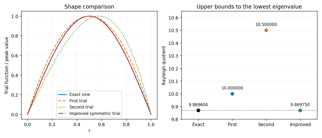
For the radial problem, set $\sigma =r\psi$. A direct differentiation gives ${\sigma }^{\prime \prime }=r{\psi }^{\prime \prime }+2{\psi }^{\prime }$, soFinite $\psi (0)$ supplies the first boundary value. The Rayleigh quotient is $R[\sigma ]={\int }_0^1{\sigma }^{\prime 2}dr/{\int }_0^1{\sigma }^{2}dr$. For the two trials, ${\sigma }_1=r(1-r)$ and ${\sigma }_2=r(1-r^2)$, the numerator-denominator pairs are $(1/3,1/30)$ and $(4/5,8/105)$, respectively. HenceThe exact eigenvalues are $n^2{\pi }^2$, so $E_{\min }={\pi }^2\simeq 9.86960$. Both trials give upper bounds by the Rayleigh-Ritz variational principle, and the first estimate is more accurate, since it is smaller. Trial admissibility uses the Dirichlet energy form for $\sigma$; the first trial's nonzero radial derivative at the origin does not invalidate this variational calculation.

To improve, add independent trial functions and minimize the quotient over their span. Here merely combining the two supplied trials gives no improvement: their two-dimensional stiffness and mass matrices areThe lowest Ritz value is still ten. Instead add the symmetric quartic $\tau =r^2(1-r{)}^2$. On the span of ${\sigma }_1,\tau$, the generalized eigenvalue problem hasIts determinant is $(E^2-112E+1008)/529200$, so the least root givesThis is strictly better than both original estimates. The symmetry obstruction in a polynomial Rayleigh-Ritz trial space explains why the cubic addition failed while the quartic helps. It is also the shifted-interval version of the polynomial Rayleigh-Ritz trial space for a one-dimensional box.

A square complex matrix $U$ is a unitary matrix when $U^{†}U=I$, so it preserves the Euclidean norm. If $Uv=\mu v$ with $v\ne 0$, then $\Vert v\Vert =\Vert Uv\Vert =|\mu |\Vert v\Vert$, giving $|\mu |=1$. For a Hermitian matrix $A=A^{†}$ and $A{e}_j={\lambda }_j{e}_j$,because the numerator equals its complex conjugate. Hence no eigenvalue of $A+iI$ is zero, proving it is invertible.

For $V=(A-iI)(A+iI{)}^{-1}$, the Hermitian conjugate is $V^{†}=(A-iI{)}^{-1}(A+iI)$. The factors and their inverses commute, since they are rational functions of $A$. Thus $V^{†}V=I$. Its action on the same eigenvectors isThese eigenvalues have modulus one. This is the Cayley transform of a Hermitian matrix in the convention that avoids the unitary eigenvalue one.

For the inverse direction, $U^{†}=U^{-1}$ givesTaking the conjugate transpose of $B=i(I+U)(I-U{)}^{-1}$ therefore yieldsThe last equality uses commutativity of the two factors. This proves that the inverse Cayley transform of a unitary matrix without eigenvalue one is Hermitian. Solving for $U$ gives $U=(B-iI)(B+iI{)}^{-1}$. An orthonormal eigenbasis of $B$ therefore diagonalizes $U$, with diagonal entries $(b_j-i)/(b_j+i)$.

The result extends even when a unitary matrix has eigenvalue one: choose $|\alpha |=1$ so that $\alpha U$ does not. There are only finitely many forbidden phases, since the matrix has finitely many eigenvalues. Diagonalizing $\alpha U$ also diagonalizes $U$ in the same basis. Thus every unitary matrix is unitarily diagonalizable.

The spectral theorem for real symmetric matrices supplies an orthonormal basis of real eigenvectors. Put these in the columns of $Q$, so $Q^{T}Q=I$ and $Q^{T}AQ=\mathrm{diag}({\lambda }_1,\dots ,{\lambda }_n)$. In the question's coordinate convention choose $O=Q^T$ and $y=Ox$. Since $x=O^{T}y$,Reorder the eigenvalues with $m$ positive, $\ell -m$ negative and $n-\ell$ zero. For nonzero eigenvalues set $z_i=\sqrt{|{\lambda }_i|}{y}_i$, and retain the remaining coordinates as $z_i=y_i$. This is an invertible real transformation $z=DOx$, where $D$ is the diagonal rescaling; the combined matrix $L=DO$ gives $z=Lx$. It giveswith the zero coordinates absent. The general allowed range is $0\le m\le \ell \le n$. The printed restriction $m\ge 1$ is not valid for every real symmetric matrix: a negative-definite or zero form has no positive square. The invariance of these counts is Sylvester's law of inertia.

For the specified form, a particularly simple change isSubtracting the first two squared coordinates verifies the identity directly, and $\det L=1$ proves invertibility. Thus $m=1$, $\ell =2$ and there is one zero direction. The final rescaling need not remain orthogonal.

Choose the Fourier transform convention $\hat{f}(k)={\int }_{\mathbb{R}}{e}^{-ikx}f(x)dx$, with inverse $(2\pi {)}^{-1}\int e^{ikx}\hat{f}(k)dk$. For absolutely integrable $f_1,f_2$, Fubini's theorem permits the substitution $s=x-y$ in the convolution transform:This proves the convolution theorem in the chosen convention.

Take $q(x)=\frac{1}{2}{e}^{-|x|}$. Splitting its transform at zero gives $\hat{q}(k)=\frac{1}{2}[(1+ik{)}^{-1}+(1-ik{)}^{-1}]=(1+k^2{)}^{-1}$. Thus the desired inverse is $q\ast q$. For $x\ge 0$, split the convolution integral at $y=0$ and $y=x$:The result is even, soDifferent normalization conventions alter the transform prefactors, which is why the convention was stated explicitly.

The homogeneous Cauchy-Euler equation has solutions $x$ and $x^{-1}$. Choose $y_L=x$, which vanishes at zero, and $y_R=x-x^{-1}$, which vanishes at one. Their Wronskian is $W(s)=y_L(s)y_R^{\prime }(s)-y_L^{\prime }(s)y_R(s)=2/s$. For a Green function integrated against the unweighted measure $ds$, continuity at $x=s$ and the jump condition $s^2[G_x{]}_{s^{-}}^{s^{+}}=1$ giveIt satisfies $L_{x}G=\delta (x-s)$ for $L=x^2{\partial }_x^2+x{\partial }_x-1$. Therefore the candidate solution isThe leading coefficient vanishes at zero, so the endpoint condition needs care. If $f$ extends continuously to $[0,1]$, this expression has limit $-f(0)$ as $x\downarrow 0$. Indeed $x^{-1}{\int }_0^{x}f(s)ds\to f(0)$ and $x{\int }_x^{1}f(s)s^{-2}ds\to f(0)$, while the remaining terms vanish. Thus the continuous zero-endpoint problem in this class requires $f(0)=0$. With that compatibility condition the formula gives both boundary values and is unique: a difference of two bounded solutions is $Ax+B/x$, whose two endpoint conditions force both constants to vanish. For incompatible forcing such as $f\equiv 1$, the bounded solution with $u(1)=0$ is $x-1$, which cannot also vanish at zero. Pointwise vanishing of $G(x,s)$ for fixed $s$ does not justify interchanging the singular endpoint limit with its integral. This issue is treated in Green kernel and endpoint compatibility for a singular Euler equation.

For the supplied compatible forcing $f(s)=s$, the integrals are $x^2/2$ and $(1-x^2)/2+\log x$. Their polynomial pieces cancel, givingDirect differentiation gives $Lu=x$, and $x\log x\to 0$ at zero. Its derivative diverges there, which is allowed because the boundary condition requires the value, not a finite derivative.