Topics (384k) Articles (398k) Users (410) Discussions (242) Comments (383) Files (13k) New article
For a closed smooth oriented four-manifold with , remove two balls to obtain , and choose an Admissible cut for a Heegaard Floer mixed map. Positivity and naturality show that the minus map of lands in , while the plus map of descends from . ThusThe coefficient of the bottom plus generator in this map, applied to , defines , up to the orientation sign, with . It vanishes unless . The construction is independent of the admissible cut by the cobordism composition and associativity laws. Two positive pieces explain the condition .
For a linear output , the second term limits the growth produced by the Hebbian term. On the averaged dynamics with , . For , positive-eigenvalue equilibria have norm and align with eigenvectors of . If inputs are centered, is their covariance matrix.
With , the squared weight norm satisfies . It moves monotonically toward without crossing it. Explicitly equals its initial value times . Persistent excitation therefore drives to ; without excitation it can remain stationary. This nonlinear normalization avoids the unbounded amplification of unmodified Hebbian learning.
For in geodesic normal coordinates, the Gauss lemma gives . Substituting into therefore yields , with . Integration along radial rays gives the displayed formula. Every coefficient is smooth at the centre. Any smooth solution of is zero for , since is constant and tends to zero at . This proves uniqueness. In this special divergence-form case , so every for is zero: the Gaussian itself solves the equation exactly on the coordinate ball. The positive Laplace-Beltrami operator instead has a metric volume-density term and a nonconstant leading amplitude.
For on scalar functions, the leading coefficient of the heat parametrix in normal coordinates is the inverse square root of the metric volume density: . The heat-kernel transport equations give . This gives the displayed diagonal expansion. The coefficient is specific to the minimally coupled scalar operator; a bundle connection or a curvature-dependent potential changes the general Laplace-type coefficients.
For the positive scalar Laplace-Beltrami operator on a compact manifold without boundary, the heat invariants are the integrated coefficients in the short-time heat kernel expansion. In particular and , with the scalar curvature. They are determined by the heat trace, hence by the spectrum with multiplicities. The leading positive coefficient recovers the dimension from .
A connected subset of Euclidean space containing distinct points has Hausdorff dimension at least one. The Lipschitz map maps onto a set containing , since continuous images of connected spaces are connected. A Lipschitz map cannot increase Hausdorff dimension, whereas an interval has Hausdorff dimension one. Consequently any set of Hausdorff dimension less than one is totally disconnected.
Suppose shrinking interval covers of have length-power sums with logarithmic growth rate , and is strictly decreasing with zero . For every those sums tend to zero exponentially. The definition of Hausdorff measure then gives , hence the displayed upper bound. A matching lower bound requires additional information and does not follow from this covering argument alone.
The middle-third Cantor set has Hausdorff dimensionIts Lebesgue measure is zero, yet . These assertions measure different aspects of size: interval length is too coarse to distinguish this set from a null set, while the critical fractional measuring rule captures its remaining structure.
At level , the construction covers by intervals of diameter . Their total -cost isFor it tends to zero, proving the upper dimension bound. At it equals one, giving . For this particular cover's cost grows, but that alone would not prove a lower bound on Hausdorff measure.
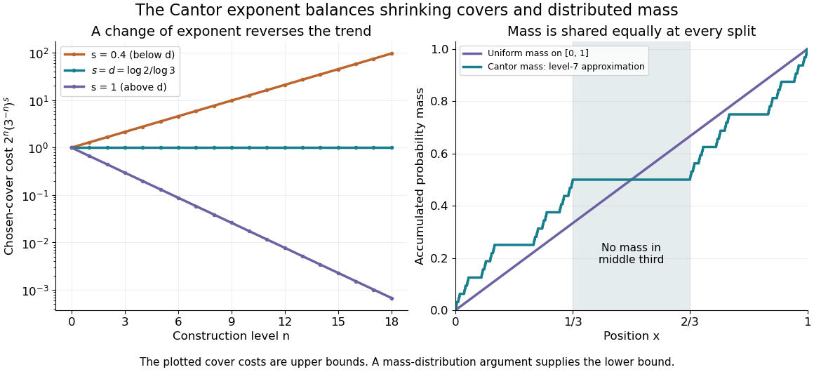
Cantor cover costs change trend at the critical exponent, and distributed mass supplies the lower bound
. Details. For the matching lower bound, use the Cantor distribution, which assigns mass to each level- Cantor cylinder. An interval of length with meets at most two level- construction intervals, since their gaps are at least . Its mass is therefore at mostEvery covering set of diameter in the line lies in an interval of length , so any small cover must have total -cost at least . This is the mass distribution principle in its interval form: , sufficient to prove the claimed dimension. The constants are convenient bounds, rather than an assertion of the exact critical Hausdorff measure. In the diagram, the right panel is a finite-stage approximation to the Cantor function, showing how probability is shared while the middle third receives none.
The reusable pattern is to obtain an upper bound by constructing covers and a lower bound by distributing mass. The same strategy underlies Cartesian powers of the Cantor set and the dimension formula for a finite similarity iterated function system satisfying the open set condition.
The mass distribution principle converts a diffuse measure into a lower bound on Hausdorff dimension. Let and let a Borel probability measure give a Borel set full mass. If, for some , every ball centered in satisfiesthen in the diameter-cost convention, and consequently .
The idea is to keep unit mass from being crowded into cheap covering pieces. For a piece of positive diameter meeting , choose . A ball of radius contains ; letting gives , where is the associated outer measure. Zero-diameter pieces have zero mass by the same estimate. For any sufficiently small cover,Thus every cover costs at least . This is the lower-bound counterpart to the explicit covers in scale-restricted Hausdorff content. The Cantor distribution supplies the needed mass in Hausdorff dimension of the Cantor set. [ref]
https://www.math.stonybrook.edu/~bishop/fractalbook.pdf. Bishop and Peres, §1.2: the mass distribution principle
. Harris theorem for square-lattice bond percolation by  Codex 0 Created 2026-10-14 Updated 2026-11-05
Uniform fixed-aspect rectangle crossing in bond percolation bounds at the self-dual parameter yield a positive lower bound for closed dual circuits in geometrically spaced disjoint annuli. The independent annular barriers for percolation imply that an origin-to-infinity open graph path has probability zero. Parameter monotonicity gives zero percolation probability for every .
For a positive harmonic function on the unit disc, choose a global harmonic conjugate and apply the Carathéodory derivative bound for the right half-plane to . This gives by the Cauchy-Riemann equations. A disk automorphism sending zero to has derivative modulus , so the chain rule gives the displayed bound. Composing a boundary-pole Poisson kernel with a disk automorphism attains equality, proving the coefficient is optimal at every point.
Planar Brownian motion started at , , exits the positive quadrant through either positive coordinate axis with probability one-half. The density along each axis is for , measured with respect to distance along that axis. Squaring maps the quadrant to the upper half-plane and sends the starting point to . The boundary square therefore has the centered Cauchy distribution of scale ; pulling it back by gives the displayed density. The radius has distribution function , independently of which axis is chosen. There is no atom at the origin.
For , the exponential growth rate of a q-ary Hamming ball is . Stirling's formula gives the exponent of each summand , and the sum lies between its largest term and times that term. Above the entropy-maximizing radius fraction, the exponent is one.
// Target: algebra.bigb
The Icosian game made the vertex-visit puzzle tangible. The report of its 1857 presentation describes a plane projection of a regular dodecahedron, with holes at the vertices for ivory pins. The Trinity College Dublin archive connects this game with the search for closed routes visiting each vertex exactly once. This puzzle supplies a historical illustration of the Hamilton cycle requirement.[ref]
The Icosian Calculus, Hamilton papers archive. The Icosian Calculus, Hamilton papers archive: opening historical introduction and quoted report of the 1857 British Association presentation: dodecahedron projection and ivory pins
A weighted Hamilton cycle is a Hamilton cycle in a weighted graph, with cost equal to the sum of its traversed edge weights. Here weights represent symmetric nonnegative costs, rather than conductances. Asking whether a Hamilton cycle exists is a feasibility question; asking for the cheapest one is an instance of the travelling salesman problem. A complete graph supplies every possible connection between distinct vertices, making feasibility automatic for , while choosing the cheapest visiting order remains a separate mathematical optimization problem.
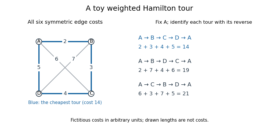
A fictitious weighted graph on four vertices: its three Hamilton cycles, identified under reversal and cyclic rotation, have costs 14, 19 and 21
. Details. Assign the complete graph the symmetric edge costs , , , , and , in arbitrary units. Fix the start at and identify each Hamilton cycle with its reverse. The three possibilities areThese exhaust the possibilities: the permutations of the other three vertices give orders, paired into three reversals. Hence the perimeter tour really is optimal for this toy instance. The diagram's geometric lengths are not costs, and no triangle inequality is assumed.
The usefulness of this model is to distinguish visiting required sites from covering required connections. If tasks are assigned to vertices and the route must return after one visit to each, a weighted Hamilton cycle captures the ordering requirement. If the job instead requires each edge once, the relevant object is an Euler circuit. The shortest path problem asks only for a cheapest route between specified endpoints. A 1954 primary research paper gave a concrete motivation for the travelling salesman problem: certify that a particular tour through 49 cities has minimum road-distance cost.[ref]
Solution of a Large-Scale Traveling-Salesman Problem by George B. Dantzig and others. Solution of a Large-Scale Traveling-Salesman Problem by G. Dantzig, R. Fulkerson and S. Johnson, abstract; Journal of the Operations Research Society of America 2(4), pp. 393–410 (1954)
These are abstract route models. If a cost stands for a whole graph path through an underlying network, travelling between consecutive task vertices can pass through intermediate network vertices more than once. One visit per task therefore does not imply one visit per physical junction. One-way connections require a directed graph; changing costs or extra timing constraints require a richer model than the fixed symmetric toy instance.
A Hamiltonian graph must be a connected graph and have minimum degree : each vertex has two distinct neighbours on its Hamilton cycle. It also has no cut vertex. Indeed, deleting any vertex from the Hamilton cycle leaves a graph path through every remaining vertex, so the remaining graph is connected. These are quick ways to rule out a Hamilton cycle.[ref]
Hamilton Cycles. Diestel, Graph Theory, §10.1, printed pp. 323–324: necessary minimum degree two and 2-connectivity
Even these conditions together are not sufficient: the complete bipartite graph is connected, has minimum degree two and no cut vertex, but has no Hamilton cycle. Every graph cycle in a bipartite graph alternates between its two parts, using equally many vertices from each; it cannot use all two and all three.
In the other direction, Dirac's theorem gives a sufficient condition: a finite simple graph with and has a Hamilton cycle. Failure of this inequality proves nothing by itself: the cycle graph has a Hamilton cycle despite .[ref]
A Hamiltonian graph is a graph containing a Hamilton cycle. This describes existence of a spanning graph cycle, rather than requiring every edge of the graph to belong to that graph cycle. In the finite simple graph convention, is a Hamiltonian graph for , because any ordering of its vertices closes using available edges.
The Hall coefficient relates a transverse electric field to longitudinal current density and transverse magnetic field, with oriented axes as in the displayed formula. Its SI unit is . For one isotropic Drude model species it is ; multiple charge carriers need not follow that formula.
For a finite nonempty integer set , put . If an integer , some of size at least has a Freiman 2-isomorphism into . Choose an auxiliary prime so large that reduction is injective on and every nonzero element of remains nonzero. Dilate modulo by a uniformly chosen nonzero multiplier. The forbidden residues are those represented by nonzero multiples of of absolute value less than , at most residues. The nonzero elements of occur in opposite pairs; the two elements in each pair have the same bad event. The union bound therefore gives failure probability at most . Choose a multiplier avoiding all these events. Select the more populated of two half-intervals of residues modulo . Differences of two pair sums of representatives then have absolute value less than . An original additive relation must therefore lift to equality in the integers; conversely an equality modulo cannot have a nonzero lifted difference, by the forbidden-residue choice. Reduction modulo is the required isomorphism.
Pinned article: Introduction to the OurBigBook Project
Welcome to the OurBigBook Project! Our goal is to create the perfect publishing platform for STEM subjects, and get university-level students to write the best free STEM tutorials ever.
Everyone is welcome to create an account and play with the site: ourbigbook.com/go/register. We belive that students themselves can write amazing tutorials, but teachers are welcome too. You can write about anything you want, it doesn't have to be STEM or even educational. Silly test content is very welcome and you won't be penalized in any way. Just keep it legal!
Intro to OurBigBook
. Source. We have two killer features:
- topics: topics group articles by different users with the same title, e.g. here is the topic for the "Fundamental Theorem of Calculus" ourbigbook.com/go/topic/fundamental-theorem-of-calculusArticles of different users are sorted by upvote within each article page. This feature is a bit like:
- a Wikipedia where each user can have their own version of each article
- a Q&A website like Stack Overflow, where multiple people can give their views on a given topic, and the best ones are sorted by upvote. Except you don't need to wait for someone to ask first, and any topic goes, no matter how narrow or broad
This feature makes it possible for readers to find better explanations of any topic created by other writers. And it allows writers to create an explanation in a place that readers might actually find it.
Figure 1. Screenshot of the "Derivative" topic page. View it live at: ourbigbook.com/go/topic/derivativeVideo 2. OurBigBook Web topics demo. Source. - local editing: you can store all your personal knowledge base content locally in a plaintext markup format that can be edited locally and published either:This way you can be sure that even if OurBigBook.com were to go down one day (which we have no plans to do as it is quite cheap to host!), your content will still be perfectly readable as a static site.
- to OurBigBook.com to get awesome multi-user features like topics and likes
- as HTML files to a static website, which you can host yourself for free on many external providers like GitHub Pages, and remain in full control

Figure 2. You can publish local OurBigBook lightweight markup files to either OurBigBook.com or as a static website.
Figure 3. Visual Studio Code extension installation.
Figure 5. . You can also edit articles on the Web editor without installing anything locally. Video 3. Edit locally and publish demo. Source. This shows editing OurBigBook Markup and publishing it using the Visual Studio Code extension. 
- Infinitely deep tables of contents:




All our software is open source and hosted at: github.com/ourbigbook/ourbigbook
Further documentation can be found at: docs.ourbigbook.com
Feel free to reach our to us for any help or suggestions: docs.ourbigbook.com/#contact