Topics (384k) Articles (398k) Users (410) Discussions (242) Comments (383) Files (13k) New article

The Itô formula identifies the operator of an SDE with drift and noise vector fields as the displayed second-order operator. With bounded measurable coefficients, every solution satisfies the true martingale identity for test functions, hence is an L-diffusion in the martingale-problem sense.
// Target: probability-and-statistics.bigb
Couple with and the same initial value. If has Lipschitz constant , the Gronwall inequality gives . Applying the Gaussian maximal bound for Brownian motion coordinatewise in dimension bounds the deviation probability by for . Matching initial values is essential.
For a centered scalar normal random variable of variance , the Isserlis theorem sums complete pairings of factors. The first factor has partners, then choices remain for the first unpaired factor, giving . Odd moments vanish. Summing the moment-generating function gives . This is a scalar formula, not a formula for the length of a vector.
Boyle's law states that a fixed amount of substance of an ideal gas at constant absolute thermodynamic temperature has constant product of absolute pressure and total volume:Here is measured relative to a vacuum, not relative to the surrounding atmospheric pressure. Halving the volume doubles the absolute pressure; doubling the volume halves it. A real gas approximately follows Boyle's law when it is sufficiently dilute and far from a phase transition.[ref]
2.1 Molecular Model of an Ideal Gas. §2.1, The Gas Laws, Figure 2.4, and equations 2.1–2.2: fixed temperature and particle number, absolute pressure, and the dilute-gas limit
For an original calculated example, suppose a sealed gas sample has and . After isothermal compression to ,Both states have , since . The volume ratio is dimensionless, so using the same volume units in numerator and denominator leaves the pressure in kilopascals. Although has units of energy, its value is not the compression work: isothermal ideal-gas work involves an integral along the path.
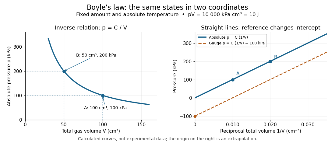
The blue curves show calculated ideal gas states, not measurements. The left panel is a branch of a hyperbola; the right panel plots exactly the same absolute pressures against . The dashed line uses gauge pressure with a stipulated constant atmospheric pressure of . Its displaced intercept explains why absolute pressure in Boyle's law matters.
A short derivation starts from the ideal gas law, . Fixing the amount of substance and absolute thermodynamic temperature fixes , where is the molar gas constant. The microscopic picture in ideal gas pressure from wall collisions is equally appealing: at fixed temperature, the typical particle kinetic energy stays fixed, while compression increases the number density and wall momentum transfer per unit surface area and time. A larger absolute pressure follows without requiring hotter particles.
The constraints are essential. A leak changes the amount of substance. Rapid compression can raise the temperature before heat transfer restores thermal equilibrium, as in the isothermal gas syringe experiment. Molecular size and interactions in a dense real gas invalidate the ideal gas approximation; the Van der Waals equation describes one such correction. Equal endpoint temperatures allow an endpoint test of Boyle's law, but do not establish that every intervening state lies on an isothermal process.
For fixed mass , mass density satisfies , so it is proportional to absolute pressure. In a dilute bubbly flow, Boyle's law allows bubble volume and its contribution to buoyancy to increase as hydrostatic pressure decreases, provided gas mass is retained, dissolution is negligible, and the temperature stays approximately fixed. Its usefulness is that a simple ratio predicts a substantial size change without tracking individual molecules.
Why must a conducting piston move slowly? A simple model couples the first law of thermodynamics to Newton's law of cooling. Assume a fixed amount of ideal gas with uniform temperature and constant whole-sample heat capacity at constant volume , a heat bath maintained at , negligible friction, and mechanically slow motion. Let be the effective thermal conductance, the reciprocal of the thermal resistance, in . ThenPositive heat transfer must offset expansion work to keep near . A finite and nonzero piston speed therefore require a temperature difference. This uniform-temperature model neglects spatial temperature gradients, sensor response, cylinder heat capacity and any change of with piston position; it is an illustrative calculation, not a fit to the isothermal gas syringe experiment.
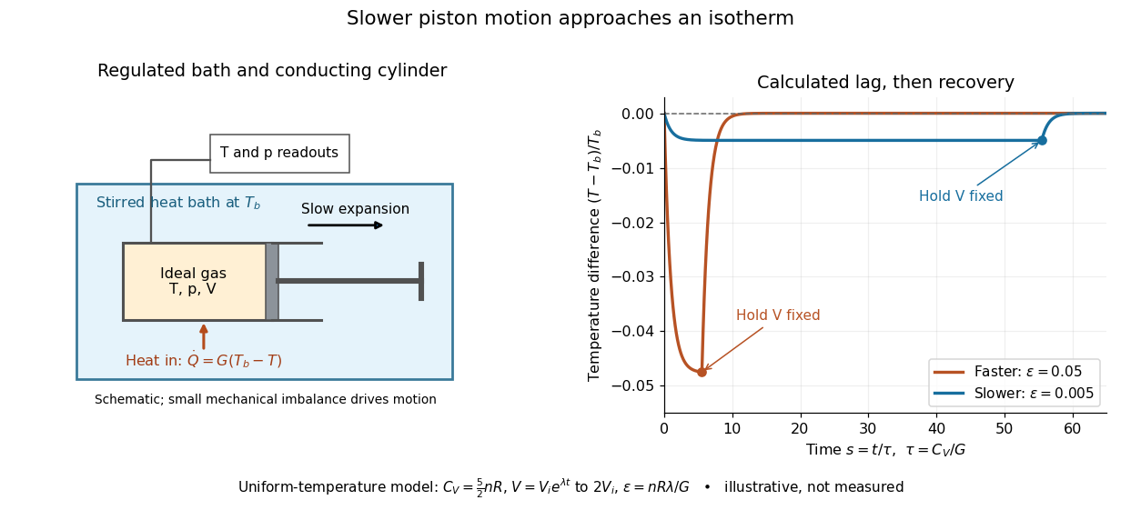
Conducting piston in a thermal bath and modeled temperature lag during expansion
. Details. For a prescribed exponential volume change , define , and . The dimensionless temperature obeys a linear ordinary differential equation with initial value :The plotted expansion uses stipulated and stops at , at . During expansion, the larger produces the larger temperature deficit; once the piston is held fixed, the deficit undergoes exponential decay as . Reducing makes the path more nearly an isothermal process, while increasing its duration. Reversing the piston with produces a temperature excess and outward heat transfer; the small- regime is the intended near-isothermal approximation. Mechanical slowness alone does not ensure sufficient heat transfer.
For a reversible thermodynamic process that changes the volume of a fixed amount of ideal gas at absolute temperature , the work done by the gas isHere is the amount of substance, the molar gas constant, the pressure, and the natural logarithm. The ideal gas law supplies ; the integral is the signed area under the pressure-volume curve. Isothermal expansion gives positive work; isothermal compression gives negative work. A convention counting work done on the gas instead has .[ref]
For a calculated example, let , and , . The pressure falls from approximately to , andTraversing the same isothermal process backward changes both transfer signs: . Neither direction changes internal energy of an ideal gas. These stipulated values illustrate the energy balance; they are not experimental measurements.
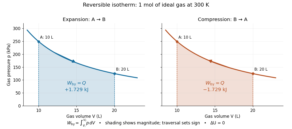
The shaded geometric area is positive in both panels; the direction of the integral supplies the sign of work. Knowing only the two equilibrium endpoints does not justify shading this curve for an irreversible process. For an idealized piston moving against a specified external resisting pressure, boundary work is . Substitution of the equilibrium gas pressure requires the appropriate reversible limit. In free expansion into vacuum, and this boundary work is zero.
With positive ladder coefficients, the second-axis half-turn is . Conjugation sends to , making consecutive phases differ by a minus sign. The highest-state rotation formula, expanded through its last nonzero lowering term, fixes the highest-state phase to one.
An isospin-invariant decay amplitude is an intertwining map from the initial isospin multiplet into the final tensor product. The Clebsch-Gordan decomposition for SU2 contains each allowed final isospin once. Commutation with the third generator and the quadratic Casimir operator places the image in the matching coupled state. Commutation with the ladder operators makes its scalar coefficient independent of the magnetic component. Orthogonality of the Clebsch-Gordan coefficients then gives a summed squared amplitude . A physical decay rate additionally includes phase space and spin sums, which can be absorbed into a common reduced coefficient when exact isospin symmetry makes them identical between channels.
A finite group presentation has a recursive upper bound on its Dehn function exactly when its word problem for a group is decidable. If the maximal relator length is and a word has length , a diagram of area at most can be chosen with at most edges. Enumerating all finite labelled planar diagrams within that bound gives a terminating test. Conversely, a word decider identifies the finitely many null words of length at most ; exhaustive finite diagram searches find their minimal areas, whose maximum computes the Dehn function.
The IP-star sets form a proper filter on a set over the positive integers. Indeed, sets that are not IP sets are closed under taking subsets. They are also closed under finite unions, because the partition regularity of IP sets would otherwise put an IP set in one of the union's constituent sets. Taking complements gives upward closure and closure under finite intersections for the IP-star sets. The full set belongs to this filter and the empty set does not.
For terminal logarithmic utility and running logarithmic utility , with , constant Black-Scholes model coefficients give and , where is the state-price density. The optimal terminal wealth and consumption are and . Their discounted budget adds to . The concave supporting-tangent inequality, integrated over time, proves optimality; the Itô formula gives the displayed dollar stock holding. The time-dependent consumption-to-wealth ratio reflects both remaining consumption opportunities and the terminal utility weight.
For constant relative risk aversion utility with parameter , terminal weight and utility discount rate , in a Black-Scholes model put , and . The displayed optimal consumption and dollar stock position follow by inverse marginal utility and the state-price budget constraint. For the value is with discount measured from . Finite horizons do not require . The concave supporting-tangent inequality and replication of the optimal budget prove global optimality, rather than only a formal differential-equation solution.
For the inverse Gaussian sum closure, take . The saddle solves , and . Substitution in the saddlepoint density approximation givesThis is the exact sum density, so its leading saddlepoint expression needs no correction or renormalization.
Let be conditionally independent inverse-gamma distribution observations with known shape , unknown scale , and observed values . Their likelihood function isA gamma distribution prior with shape and rate is a conjugate prior, givingThis follows by multiplying the two powers of and the two exponential factors. It uses reciprocal observations, rather than their sample mean.
If , the conditional claim expected value is . Its Bayes estimator under squared error loss is the posterior expected valueHere the target is the conditional expected value, whose posterior second moment is finite because the posterior for is gamma. When , the conditional claim expected value is infinite and this finite-estimate formula does not apply. For example, , , and observations give posterior shape , rate , and estimated conditional claim expected value .
For the continuously differentiable inverse function supplied by the inverse function theorem, the chain rule applied to givesHere is the identity matrix. The matrix inverse is taken at the recovered input , not at the output . In one dimension this is the inverse function rule .
The formula also describes sensitivity. For a small output perturbation , differentiability gives . A large operator norm of permits large amplification in some directions. In the square root example, grows without bound as positive approaches zero. Existence of a local inverse function therefore does not imply that recovery is insensitive to measurement error.
For a real sequence of exchangeable random variables, every event in its invariant sigma-algebra of an exchangeable sequence agrees almost surely with an event of its tail sigma-algebra. Put . Approximate in by its conditional expectation on the first coordinates. Swap that block with the next coordinates. Invariance of and the law shows that the conditional expectation on the second block is an equally good approximation. It is measurable with respect to the tail after index . The L1 contraction of conditional expectation then bounds by twice the approximation error. The reverse martingale convergence theorem gives almost surely. Thresholding the latter at supplies the required tail event. Together with the reverse inclusion, the two sigma-algebras have identical probability completions.
For , a meromorphic function satisfying the modular transformation law is a cusp form exactly when its invariant norm is bounded. The bound first excludes interior poles. At each cusp a genuine periodic slash translate is bounded by , which tends to zero. Its punctured-disk expression therefore has a removable singularity with zero value. Conversely cusp Fourier expansions decay exponentially, and finitely many compact core regions control the rest. Positive weight is essential: a nonzero constant in weight zero satisfies the bound but is not a cusp form.
Interval subdivision covers by smaller closed intervals , computes a valid interval enclosure on each, and takes their union. Every allowed input belongs to a piece, so its output belongs to that union. If one closed interval is wanted, take the smallest one containing the union; gaps between separate output pieces can then be lost. Splitting narrows the freedom given to repeated inputs, while increasing the number of evaluations.
For , split at . The natural interval extensions areTheir union is . Four equal pieces sharpen the upper bound again:The union is now , still wider than the actual image of a function . These are exact rational number bounds: the excess width comes from the interval dependency problem, rather than roundoff error.
A smooth point of an algebraic plane curve is a flex if its tangent line has intersection multiplicity at least three there. This definition also applies to smooth points of a singular curve.
Pinned article: Introduction to the OurBigBook Project
Welcome to the OurBigBook Project! Our goal is to create the perfect publishing platform for STEM subjects, and get university-level students to write the best free STEM tutorials ever.
Everyone is welcome to create an account and play with the site: ourbigbook.com/go/register. We belive that students themselves can write amazing tutorials, but teachers are welcome too. You can write about anything you want, it doesn't have to be STEM or even educational. Silly test content is very welcome and you won't be penalized in any way. Just keep it legal!
Intro to OurBigBook
. Source. We have two killer features:
- topics: topics group articles by different users with the same title, e.g. here is the topic for the "Fundamental Theorem of Calculus" ourbigbook.com/go/topic/fundamental-theorem-of-calculusArticles of different users are sorted by upvote within each article page. This feature is a bit like:
- a Wikipedia where each user can have their own version of each article
- a Q&A website like Stack Overflow, where multiple people can give their views on a given topic, and the best ones are sorted by upvote. Except you don't need to wait for someone to ask first, and any topic goes, no matter how narrow or broad
This feature makes it possible for readers to find better explanations of any topic created by other writers. And it allows writers to create an explanation in a place that readers might actually find it.
Figure 1. Screenshot of the "Derivative" topic page. View it live at: ourbigbook.com/go/topic/derivativeVideo 2. OurBigBook Web topics demo. Source. - local editing: you can store all your personal knowledge base content locally in a plaintext markup format that can be edited locally and published either:This way you can be sure that even if OurBigBook.com were to go down one day (which we have no plans to do as it is quite cheap to host!), your content will still be perfectly readable as a static site.
- to OurBigBook.com to get awesome multi-user features like topics and likes
- as HTML files to a static website, which you can host yourself for free on many external providers like GitHub Pages, and remain in full control

Figure 2. You can publish local OurBigBook lightweight markup files to either OurBigBook.com or as a static website.
Figure 3. Visual Studio Code extension installation.
Figure 5. . You can also edit articles on the Web editor without installing anything locally. Video 3. Edit locally and publish demo. Source. This shows editing OurBigBook Markup and publishing it using the Visual Studio Code extension. 
- Infinitely deep tables of contents:




All our software is open source and hosted at: github.com/ourbigbook/ourbigbook
Further documentation can be found at: docs.ourbigbook.com
Feel free to reach our to us for any help or suggestions: docs.ourbigbook.com/#contact