For a stationary internal gravity wave in constant buoyancy frequency $N$ and wind $U=U_0(1+z/H)$, set $q_0=k{U}_0/N<1$. Its upward group velocity has ratio $dx/dz=k/m=q/\sqrt{1-q^2}$, where $q=q_0(1+z/H)$. Integrating from the origin gives a circular ray with center $(H\sqrt{1-q_0^2}/q_0,-H)$ and radius $H/q_0$. The ascending ray becomes horizontal at the turning level of a stationary internal wave; its reflected branch continues downwind along the same circle.

A continuous function on any real interval has image a real interval. Given two image values and an intermediate value, choose preimages and apply the intermediate value theorem on the closed segment joining them, which stays inside the domain. Neither compactness nor boundedness of the original interval is needed. In particular $f(x)=\sin (1/x)/x$ on $(0,1]$ is a continuous surjection onto $\mathbb{R}$: its values are unbounded above and below, so its interval image contains every real number.

For a short proof outline, endpoint values give the non-strict cases immediately. If $y$ is strictly between $f(a)$ and $f(b)$, apply the bisection method to the continuous function $g(x)=f(x)-y$. A midpoint with $g=0$ finishes the proof. Otherwise retain nested intervals $[a_k,b_k]$ with strictly opposite signs and widths $(b-a)2^{-k}$. The nested interval theorem, using completeness of the real numbers, gives a common point $c$ to which both endpoint sequences converge. After reversing the sign of $g$ if necessary, $g(a_k)<0<g(b_k)$. Continuity makes both endpoint value sequences converge to $g(c)$, forcing $g(c)\le 0$ and $g(c)\ge 0$, hence $f(c)=y$. The original endpoint values differ from $y$, so $c\in (a,b)$. This proof explains why a jump can defeat the construction: shrinking a candidate closed interval cannot supply the missing continuity.

Consider the original worked example $f(x)=x^3+x-1$ on $[0,1]$. First, existence: a polynomial function is a continuous function, and $f(0)=-1<0<1=f(1)$. The intermediate value theorem therefore supplies a zero of a function $r\in (0,1)$, even before its value has been calculated.

Second, uniqueness is a separate argument. The derivative is $f^{\prime }(x)=3x^2+1>0$. The derivative criterion for monotonicity, obtained from the mean value theorem, makes $f$ a strictly increasing function. Two distinct zeros of a function would contradict that strict increase. Thus this root bracket contains exactly one zero of a function; indeed the same derivative argument proves uniqueness on the entire real line.

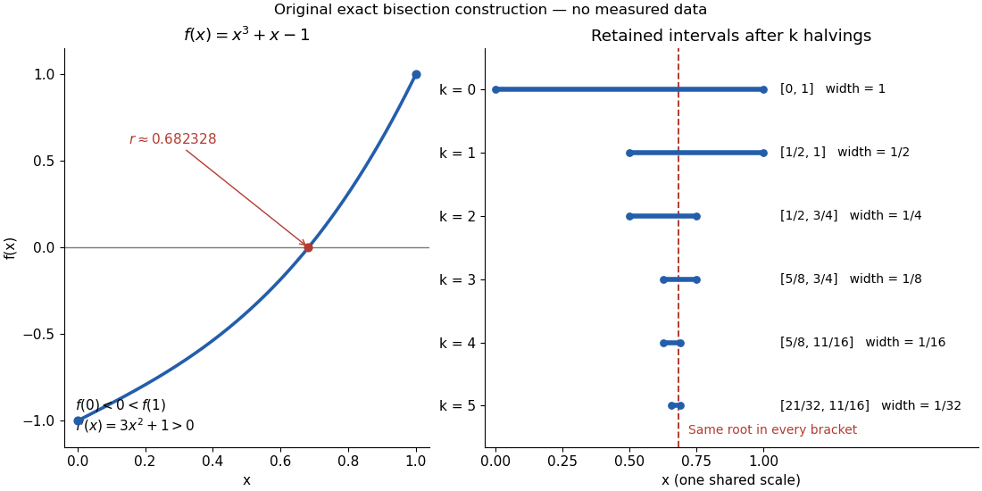
Third, localization uses the existing bisection method. Set $[a_0,b_0]=[0,1]$; after $k$ completed halvings, retain $[a_k,b_k]$ with opposite endpoint signs. Each update tests the old midpoint $m_{k-1}=(a_{k-1}+b_{k-1})/2$. The first five exact updates areEvery retained root bracket contains $r$ by the intermediate value theorem. After ten halvings, exact arithmetic givesHence $0.681640625<r<0.6826171875$. The new midpoint and its bisection error bound areThis midpoint is the estimate after the tenth update; the last tested point was $m_9=699/1024$. In general the retained width is $2^{-k}$, so the bisection error bound is $2^{-(k+1)}$. Nine halvings already suffice for an error at most $10^{-3}$, since $2^{-10}=0.0009765625<10^{-3}$. This guarantee comes from the width of the root bracket, independently of any displayed decimal approximation to the unknown zero of a function. Endpoint signs must be established reliably if evaluations use floating-point arithmetic.

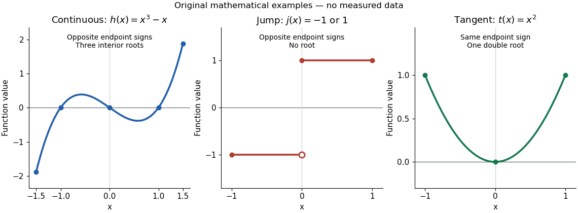
Three explicit functions separate the hypotheses from the conclusion. These are original mathematical illustrations, not measured data.

The polynomial function $h(x)=x^3-x=x(x-1)(x+1)$ is a continuous function on $[-3/2,3/2]$, with $h(-3/2)=-15/8$ and $h(3/2)=15/8$. The intermediate value theorem guarantees at least one zero of a function in the interior, while the polynomial factorization displays three: $-1,0,1$. Thus strict opposite signs do not establish uniqueness.

The everywhere-defined functionhas $j(-1)=-1$ and $j(1)=1$, yet no zero of a function. Its jump discontinuity at zero is exactly where the continuity hypothesis fails. A drawn vertical connector would be misleading: the function graph contains neither the intermediate heights nor a zero of a function at that jump. Even continuity only on the interior is insufficient: setting $q(x)=-1$ for $0\le x<1$ and $q(1)=1$ gives opposite endpoint signs on $[0,1]$ with no zero of a function, because the left one-sided limit at $1$ is not $q(1)$.

The polynomial function $t(x)=x^2$ on $[-1,1]$ is a continuous function, and $t(-1)=t(1)=1$, yet $t(0)=0$. Its root of a polynomial at zero has multiplicity of a root two. The function graph touches its horizontal tangent line there and stays positive on both sides: existence of a zero of a function does not require a sign change. More generally, near a real root of a polynomial $r$, a polynomial factorization $p(x)=(x-r{)}^{2m}u(x)$ with $m\ge 1$ and $u(r)\ne 0$ has the same sign on both sides sufficiently close to $r$, since the continuous function $u$ retains its sign. The intermediate value theorem does not rule out values outside the range between endpoint outputs.^[ref]

For a connected source, first integrate on its universal covering Lie group. The resulting map descends to the original group exactly when it kills the discrete kernel of the covering map. For the circle group, a real-linear map $t\mapsto ct$ integrates to a circle endomorphism exactly when $c\in \mathbb{Z}$, since $2\pi \mathbb{Z}$ must map into itself. This is a global period condition invisible to the zero bracket of the circle's Lie algebra.

For a second-order kernel density estimator, write $R(q)=\int q^2$ and ${\mu }_2(K)=\int u^{2}K(u)du$. Under the usual smoothness and shrinking-bandwidth assumptions, the leading mean integrated squared error is the displayed sum of integrated variance and squared bias of an estimator. Its minimizer is $h=[R(K)/(n{\mu }_2(K{)}^{2}R(f^{\prime \prime })){]}^{1/5}$, giving order $n^{-4/5}$. An added $O(n^{-1})$ integrated covariance term is lower order at this bandwidth and does not change its leading constant.

For a nonnegative nonincreasing function $f:[1,\infty )\to [0,\infty )$, comparison with unit-width rectangles givesOn $[n,n+1]$, the function is at most $f(n)$; on $[n-1,n]$, it is at least $f(n)$. Summing these inequalities gives the bounds. Applying them to $f(x)=1/x$ gives $\log (N+1)\le H_N\le 1+\log N$ for the harmonic numbers. Unlike a convergence verdict alone, the finite bounds estimate the size of a partial sum.

Under injective linear modelling of a small sumset, every $w\in W$ has a unique lift $\sigma (w)\in 4B$, because differences of two lifts lie in $8B\subseteq 12B$. For $w_1,w_2\in W$, the discrepancy $\sigma (w_1)+\sigma (w_2)+\sigma (w_1+w_2)$ lies in $12B\cap \ker L$, so it is zero. Thus $\sigma$ is a linear map and its image is a vector subspace of the same size as $W$. This verifies the additive lifting step rather than assuming that a preimage chosen from a sumset is automatically a subspace.

The word "projection" does not mean ordinary perpendicular projection in the plotted Euclidean space. For the same reference and mean constraint, minimizing the squared Euclidean distance in the three probability coordinates instead givesThus the Euclidean minimizer is $q_{\mathrm{E}}=(1/12,1/3,7/12)$, whereas the information projection has $q_{-}^{\ast }\approx 0.116204$. The squared Euclidean objective at its own minimum is $1/8$; its relative entropy is approximately $0.210918$ nats, larger than the optimum $0.197378$ nats. Both distributions satisfy the same constraint.

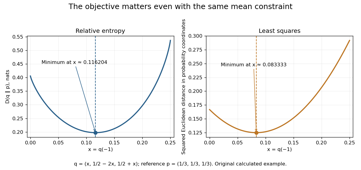
The reference and objective encode what "least change" means. Relative entropy is asymmetric and is not a metric; its minimization answers a different question from linear least squares. The useful geometric analogy comes from a Pythagorean inequality for information projection, rather than from an assertion that the colored contours are circles.

For any real constant $c$, one-dimensional Brownian motion repeatedly returns to zero. Consider successive segments from zero until exiting $(-1,1)$, separated by returns to zero. Their capped durations are independent identically distributed positive bounded random variables by the Strong Markov property, so their sum diverges by the strong law of large numbers. On each such segment $e^{c{B}_s}\ge e^{-|c|}$. Thus the exponential clock has infinite lifetime, despite arbitrarily deep negative excursions.

Choose a maximal Brauer pair $(D,b_D)$ for the block. Its inertial quotient is $N_G(D,b_D)/(D{C}_G(D))$, and its order is the inertial index. For cyclic $D$ of order $q$, this is a prime-to-$p$ divisor of $p-1$. The number of edges of the block's Brauer tree is this index, and the exceptional multiplicity is $(q-1)/e(B)$.

For $N◃G$, $\theta \in \mathrm{Irr}(N)$ and $T=I_G(\theta )$, induction gives the displayed bijection. The inverse takes the $\theta$-isotypic component of an irreducible $G$-module, viewed as a $T$-module. Induction produces distinct $N$-isotypic components indexed by $G/T$. Any nonzero $G$-submodule meets one of them and hence, by translation and irreducibility over $T$, contains them all. The same argument shows that the inverse component is irreducible and determines the original inducing module uniquely.

For two independent uniform valuations on $[0,1]$, optimal posted price revenue is $2/(3\sqrt{3})$, attained at $p=1/\sqrt{3}$. An English auction without reserve earns the expected minimum, $1/3$. With reserve $r\in [0,1]$, revenue is $r\mathrm{Pr}(\text{exactly one valuation exceeds }r)$ plus the expected smaller valuation when both exceed $r$, namely $1/3+r^2-4r^3/3$. It is maximized at $r=1/2$, giving $5/12$. Different reserve-dependent allocation probabilities explain why this differs from the no-reserve revenue without violating revenue equivalence.

The independent private values model is symmetric when bidders have identical roles and draw their valuations independently from the same distribution. For revenue equivalence in the usual single-object setting, bidders additionally have risk neutrality and quasilinear utility. Under a strictly increasing symmetric equilibrium bidding rule, a type $v$ wins with probability $F(v{)}^{n-1}$.

// Target: mathematical-optimization.bigb

For a horizontal field $B(z)e_x$ in constant downward gravity, equilibrium obeys $(p+B^2/(2{\mu }_0){)}_z=-\rho g$. The displacement energy reduces to the displayed quadratic form. Perturbations independent of the field direction do not bend magnetic field lines and therefore have no magnetic tension penalty: an increasing mass density with height permits instability. A nonincreasing mass density gives nonnegative energy for all admitted incompressible perturbations. Along-field variation adds magnetic tension proportional to wavenumber squared, stabilizing sufficiently short waves when buoyancy is unfavorable.

A projective bundle with fibre ${\mathbb{P}}^{15}$ over the four-dimensional Grassmannian $\mathrm{Gr}(2,4)$. The condition of containing a fixed line imposes four independent linear conditions on the twenty cubic coefficients. The projection to ${\mathbb{P}}^{19}$ is proper. The line $\{x_2=x_3=0\}$ is an isolated point over $x_0^2{x}_2+x_1^2{x}_3$; isolated fibre point forces dominance in equal dimensions then proves that every cubic surface contains a line.

For an initial mass function $dN\propto m^{-\alpha }dm$ on $0.1<m/M_{\odot }<100$, complete loss of material initially above $10M_{\odot }$ removes fractionThe impulsive disruption by stellar mass loss threshold is $F=1/2$, with unique finite root $\alpha \simeq 1.79101236$. Decreasing $\alpha$ shifts mass to larger stars and increases $F$, so the idealized system is globally unbound for $\alpha <{\alpha }_{\mathrm{crit}}$. The derivation requires rapid, well-mixed loss and absence of a confining external potential.

In the local incompressible weak-field limit, take an axisymmetric wavevector $(k_r,0,k_z)$ and ${\omega }_A=\mathbf{k}\cdot \mathbf{B}/\sqrt{{\mu }_0\rho }$. Eliminating the pressure projects the radial force by $k_z^2/k^2$. This yields the displayed dispersion relation, where $\kappa$ is the radial epicyclic frequency. For a hydrodynamically stable rotation profile with outward-decreasing angular velocity, instability requires $0<{\omega }_A^2<-(k_z^2/k^2)d{\Omega }^2/d\ln r$. A purely toroidal field has no axisymmetric local field-line-bending frequency and therefore no ordinary weak-field MRI in this approximation.

For local cylindrical shear $q=-d\ln \Omega /d\ln r$ with $0<q<2$, maximizing the positive squared-growth root of the ideal magnetorotational dispersion relation gives the displayed formulas. For a Keplerian disk these are $s_{\max }=3\Omega /4$ and ${\omega }_A^2=15{\Omega }^2/16$. Field strength selects the fastest wavelength, while the maximum ideal rate is set by shear. Finite domains and magnetic diffusion can exclude that wavelength.