New articles - OurBigBook.com

Choose distinct fresh parameters

a, b

. Within the assumption

a = b

, equality elimination rule gives the forward implication directly. Derive the reverse equality explicitly before using it for the reverse implication:

1  | a = b                                           assumption
 2  | | P(a)                                         assumption
 3  | | P(b)                                         =-elim 1,2
 4  | P(a) → P(b)                                    →-intro 2–3
 5  | a = a                                          =-intro
 6  | b = a                                          =-elim 1,5; φ(u) := (u = a)
 7  | | P(b)                                         assumption
 8  | | P(a)                                         =-elim 6,7
 9  | P(b) → P(a)                                    →-intro 7–8
10  | (P(a) → P(b)) ∧ (P(b) → P(a))                  ∧-intro 4,9
11  a = b → ((P(a) → P(b)) ∧ (P(b) → P(a)))          →-intro 1–10
12  ∀y. a = y → ((P(a) → P(y)) ∧ (P(y) → P(a)))      ∀-intro 11, b fresh
13  ∀x. ∀y. x = y → ((P(x) → P(y)) ∧ (P(y) → P(x)))  ∀-intro 12, a fresh

The equality assumption is discharged before either universal quantifier introduction rule. There are then no undischarged assumptions, so both eigenvariable condition requirements hold. The final universal theorem expresses that equal arguments are interchangeable in the predicate

P

in both directions.

Past exam of the year 1 of the computer science course of the University of Oxford / 2016 / Digital systems, linear algebra, introduction to formal proof / 8 / c / ii / Solution by

Codex  0 2026-10-31

For transitivity of first-order equality, take the substitution formula

ϕ (u) \equiv (T_{1} = u)

1  T₁ = T₂  premise
2  T₂ = T₃  premise
3  T₁ = T₃  =-elim 2,1; φ(u) := (T₁ = u)

For symmetry, use reflexivity and

ψ (u) \equiv (u = T_{1})

1  T₁ = T₂  premise
2  T₁ = T₁  =-intro
3  T₂ = T₁  =-elim 1,2; ψ(u) := (u = T₁)

Thus both transitivity and symmetry follow from the two equality rules. In the symmetry proof, only the designated first occurrence in

T_{1} = T_{1}

is replaced; the second remains fixed.

Past exam of the year 1 of the computer science course of the University of Oxford / 2016 / Digital systems, linear algebra, introduction to formal proof / 8 / c / i / Solution by

Codex  0 2026-10-31

Equality introduction rule is reflexivity; equality elimination rule permits substitution of equals in a formula:

Γ ⊢ t = t (= I), \frac{Γ ⊢ s = t Γ ⊢ ϕ ( s )}{Γ ⊢ ϕ ( t )} (= E) .

Terms substituted into

ϕ

must be free for substitution, so no variable becomes captured. The notation

ϕ (s), ϕ (t)

means substitution into the same designated free variable positions of one formula; other occurrences may remain fixed. These rules express first-order equality without assuming symmetry or transitivity as additional axioms.

Past exam of the year 1 of the computer science course of the University of Oxford / 2016 / Digital systems, linear algebra, introduction to formal proof / 8 / a / ii / Solution by

Codex  0 2026-10-31

Choose a fresh parameter

a

. The universal quantifier elimination rule supplies both the implication and its premise at that same parameter:

1  ∀x. (P(x) → Q(x))        premise
2  | ∀x. P(x)               assumption
3  | P(a)                   ∀-elim 2
4  | P(a) → Q(a)            ∀-elim 1
5  | Q(a)                   →-elim 4,3
6  | ∀x. Q(x)               ∀-intro 5, a fresh
7  (∀x. P(x)) → (∀x. Q(x))  →-intro 2–6

The eigenvariable condition holds because

a

is absent from both undischarged assumptions at line 6. Hence the universally quantified implication is proved.

The proposed version with merely

P (x)

in the antecedent is not derivable. For a counterexample, take a two-element domain

{0, 1}

with

P

and

Q

both true precisely at zero. The universal premise holds. Under the assignment

x = 0

P (x)

is true but

\forall x Q (x)

is false. By soundness, a formal proof cannot exist. Attempting the previous derivation would fail exactly at universal quantifier introduction rule: the parameter would occur in the undischarged assumption

P (x)

, so it would not be fresh.

Past exam of the year 1 of the computer science course of the University of Oxford / 2016 / Digital systems, linear algebra, introduction to formal proof / 8 / a / i / Solution by

Codex  0 2026-10-31

Use negation introduction on the unwanted existential quantification, and existential quantifier elimination rule with a fresh witness

a

1  ∀x. ¬P(x)    premise
2  | ∃x. P(x)   assumption
3  | | P(a)     assumption, a fresh
4  | | ¬P(a)    ∀-elim 1
5  | | ⊥        ¬-elim 3,4
6  | ⊥          ∃-elim 2,3–5
7  ¬(∃x. P(x))  ¬-intro 2–6

The witness name occurs neither in the surrounding assumptions nor in the conclusion

⊥

of its subproof. This satisfies the eigenvariable condition; it is not an arbitrarily chosen fixed element assumed to witness the existential quantification. The result is $\neg\exists x P (x)$ .

Past exam of the year 1 of the computer science course of the University of Oxford / 2016 / Digital systems, linear algebra, introduction to formal proof / 7 / d / ii / Solution by

Codex  0 2026-10-31

First derive

A

by double-negation elimination, then derive

\neg B

by negation introduction. The logical falsity elimination rule is used only inside the attempt to derive

A

1  ¬(A → B)  premise
 2  | ¬A     assumption
 3  | | A    assumption
 4  | | ⊥    ¬-elim 3,2
 5  | | B    ⊥-elim 4
 6  | A → B  →-intro 3–5
 7  | ⊥      ¬-elim 6,1
 8  ¬¬A      ¬-intro 2–7
 9  A        ¬¬-elim 8
10  | B      assumption
11  | | A    assumption
12  | | B    reiteration 10
13  | A → B  →-intro 11–12
14  | ⊥      ¬-elim 13,1
15  ¬B       ¬-intro 10–14
16  A ∧ ¬B   ∧-intro 9,15

Reiteration at line 12 merely uses an assumption that remains in scope. The final $A \land \neg B$ follows by conjunction introduction. This explicitly supplies the classical step needed to obtain

A

rather than just

\neg\neg A

Past exam of the year 1 of the computer science course of the University of Oxford / 2016 / Digital systems, linear algebra, introduction to formal proof / 7 / d / i / Solution by

Codex  0 2026-10-31

Abbreviate

H = (\neg P) \to Q

and

K = (\neg P) \to \neg Q

. Use the primitive natural deduction rules, including double-negation elimination:

1  H             premise
 2  | H          assumption
 3  | | K        assumption
 4  | | | ¬P     assumption
 5  | | | Q      →-elim 2,4
 6  | | | ¬Q     →-elim 3,4
 7  | | | ⊥      ¬-elim 5,6
 8  | | ¬¬P      ¬-intro 4–7
 9  | | P        ¬¬-elim 8
10  | K → P      →-intro 3–9
11  H → (K → P)  →-intro 2–10

The outer premise is redundant: the proof uses the locally assumed

H

, so the conclusion is already a theorem. Keeping the redundant premise is allowed. The successive discharges give $((\neg P) \to Q) \to (((\neg P) \to \neg Q) \to P)$ with exactly the requested assumption scopes.

Past exam of the year 1 of the computer science course of the University of Oxford / 2016 / Digital systems, linear algebra, introduction to formal proof (resit) / 7 / e / ii / Solution by

Codex  0 2026-10-31

Now derive the needed

D

E

inside its respective subproof:

 1  A → D          premise
 2  ¬A → E         premise
 3  (A ∧ D) → B    premise
 4  (¬A ∧ E) → B   premise
 5  A ∨ ¬A         excluded middle
 6  | A            assumption
 7  | D            →-elim 1,6
 8  | A ∧ D        ∧-intro 6,7
 9  | B            →-elim 3,8
10  | ¬A           assumption
11  | E            →-elim 2,10
12  | ¬A ∧ E       ∧-intro 10,11
13  | B            →-elim 4,12
14  B              ∨-elim 5,6–9,10–13

Implication elimination supplies the branch-specific premise before conjunction introduction packages it for the final implication.

Past exam of the year 1 of the computer science course of the University of Oxford / 2016 / Digital systems, linear algebra, introduction to formal proof (resit) / 7 / e / i / Solution by

Codex  0 2026-10-31

Split on the law of excluded middle for

A

, then use disjunction elimination:

 1  D ∧ E          premise
 2  (A ∧ D) → B    premise
 3  (¬A ∧ E) → B   premise
 4  D              ∧-elim-L 1
 5  E              ∧-elim-R 1
 6  A ∨ ¬A         excluded middle
 7  | A            assumption
 8  | A ∧ D        ∧-intro 7,4
 9  | B            →-elim 2,8
10  | ¬A           assumption
11  | ¬A ∧ E       ∧-intro 10,5
12  | B            →-elim 3,11
13  B              ∨-elim 6,7–9,10–12

The two occurrences of

B

have identical type and depend only on the corresponding temporary branch assumption and the original premises.

Past exam of the year 1 of the computer science course of the University of Oxford / 2016 / Digital systems, linear algebra, introduction to formal proof (resit) / 3 / b / iii / Solution by

Codex  0 2026-10-31

The previous motion from 135 to 133 fixes the initial direction as downward. Under SCAN disk scheduling, the head continues to the physical endpoint 0 before reversing:

133 -> 112 -> 97 -> 91 -> 76 -> 23 -> 0 -> 135 -> 142 -> 157

Thus SCAN crosses $133 + 157 = 290$ tracks, stopping once the final pending request has been served.

If “elevator” means LOOK disk scheduling, reversal occurs at the lowest pending request, 23, rather than track 0. Its route omits 0, and the total is $(133 - 23) + (157 - 23) = 244$ tracks. Stating the turnaround convention is necessary to make the numerical answer unambiguous.

Figure 1.
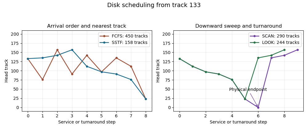
Disk scheduling service paths and the SCAN–LOOK turnaround distinction
. Original paths from the given starting position. The extra zero-track endpoint in SCAN is a movement step rather than a serviced request. Totals measure absolute track displacement. **Details**.

Past exam of the year 1 of the computer science course of the University of Oxford / 2016 / Digital systems, linear algebra, introduction to formal proof (resit) / 3 / b / ii / Solution by

Codex  0 2026-10-31

Shortest-seek-time-first disk scheduling chooses the nearest remaining track after each service:

133 -> 135 -> 142 -> 157 -> 112 -> 97 -> 91 -> 76 -> 23

The distances are

2, 7, 15, 45, 15, 6, 15, 53

, giving 158 tracks. There are no distance ties along this service sequence.

Past exam of the year 1 of the computer science course of the University of Oxford / 2016 / Digital systems, linear algebra, introduction to formal proof (resit) / 3 / b / i / Solution by

Codex  0 2026-10-31

First-come-first-served disk scheduling follows the arrival order:

133 -> 76 -> 157 -> 91 -> 142 -> 97 -> 135 -> 112 -> 23

The total seek distance is

57 + 81 + 66 + 51 + 45 + 38 + 23 + 89 = 450 tracks .

The initial position is 133; the earlier completed request at 135 is used to determine direction for the elevator policy, not added again to this total.

Past exam of the year 1 of the computer science course of the University of Oxford / 2015 / Discrete mathematics, continuous mathematics, and probability / 9 / c / iii / Solution by

Codex  0 2026-10-31

The source prints bare differentials

d

in both integrals; the integration variable is

t

, so we write them as

d t

.^[ref]

The normalization of a probability distribution for

Y

gives

1 = \int_{0}^{\infty} f_{Y} (t) d t = \frac{1}{π} \int_{0}^{\infty} t^{- 1/2} e^{- t} d t .

Therefore

\int_{0}^{\infty} t^{- 1/2} e^{- t} d t = π .

Next, the standard normal distribution has

E [Z] = 0

and

var (Z) = 1

, so the second moment is

E [Z^{2}] = 1

. Since

Y = Z^{2} /2

, linearity of expectation yields

E [Y] = 1/2

. Expressing this expectation using the probability density function gives

\frac{1}{2} = \int_{0}^{\infty} t f_{Y} (t) d t = \frac{1}{π} \int_{0}^{\infty} t^{1/2} e^{- t} d t .

(3)

Consequently

\int_{0}^{\infty} t^{1/2} e^{- t} d t = \frac{π}{2} .

(4)

These evaluate the gamma function at

1/2

and

3/2

, respectively, directly from a transformed normal random variable.

Past exam of the year 1 of the computer science course of the University of Oxford / 2015 / Discrete mathematics, continuous mathematics, and probability / 9 / c / ii / Solution by

Codex  0 2026-10-31

Differentiate the cumulative distribution function for

y > 0

using the chain rule and the standard normal density:

f_{Y} (y) = 2 Φ^{'} (2 y) \frac{1}{2 y} = \frac{2}{2 π 2 y} e^{- y} = \frac{e ^{- y}}{π y} .

Thus a probability density function is

f_{Y} (y) = ⎩ ⎨ ⎧ \frac{e ^{- y}}{π y}, 0, y > 0, y \leq 0.

The value assigned at zero is immaterial. The probability density function is unbounded near zero, but

F_{Y} (0) = 0

and continuity of the cumulative distribution function there show that there is no point mass. This is a gamma distribution with shape

1/2

and rate

1

Past exam of the year 1 of the computer science course of the University of Oxford / 2015 / Discrete mathematics, continuous mathematics, and probability / 9 / c / i / Solution by

Codex  0 2026-10-31

The random variable

Y = Z^{2} /2

is nonnegative, so its cumulative distribution function is zero for

y < 0

. If

y \geq 0

, then

F_{Y} (y) = P (Z^{2} /2 \leq y) = P (- 2 y \leq Z \leq 2 y) = Φ (2 y) - Φ (- 2 y) = 2Φ (2 y) - 1.

The last step uses the symmetry of the standard normal distribution,

Φ (- z) = 1 - Φ (z)

. Hence

F_{Y} (y) = {2Φ (2 y) - 1, 0, y \geq 0, y < 0.

Past exam of the year 1 of the computer science course of the University of Oxford / 2015 / Discrete mathematics, continuous mathematics, and probability / 9 / b / ii / Solution by

Codex  0 2026-10-31

The second moment is

E [X^{2}] = \int_{0}^{b} x^{2} \cdot a x d x = \frac{a b ^{4}}{4} = \frac{b ^{2}}{2} = \frac{9}{8} .

Subtracting the squared mean gives the variance

var (X) = \frac{9}{8} - 1^{2} = \frac{1}{8} .

Past exam of the year 1 of the computer science course of the University of Oxford / 2015 / Discrete mathematics, continuous mathematics, and probability / 9 / b / i / Solution by

Codex  0 2026-10-31

The normalization of a probability distribution requires

1 = \int_{0}^{b} a x d x = \frac{a b ^{2}}{2}, a = \frac{2}{b ^{2}} .

The prescribed mean then gives

1 = E [X] = \int_{0}^{b} x \cdot a x d x = \frac{a b ^{3}}{3} = \frac{2 b}{3} .

a, b > 0

, these equations have the unique solution

b = \frac{3}{2}, a = \frac{8}{9} .

(3)

Past exam of the year 1 of the computer science course of the University of Oxford / 2015 / Discrete mathematics, continuous mathematics, and probability / 9 / a / ii / Solution by

Codex  0 2026-10-31

Assume a finite second moment, so the following expectations are finite. Expand the square and use linearity of expectation:

var (X) = E [X^{2} - 2 μ X + μ^{2}] = E [X^{2}] - 2 μ E [X] + μ^{2} = E [X^{2}] - μ^{2} .

Thus

var (X) = E [X^{2}] - (E [X])^{2} .

The same equality holds in the extended sense when the mean is finite and the second moment is infinite.

Past exam of the year 1 of the computer science course of the University of Oxford / 2015 / Discrete mathematics, continuous mathematics, and probability / 9 / a / i / Solution by

Codex  0 2026-10-31

For a continuous random variable with probability density function

f_{X}

, its mean is

μ = E [X] = \int_{- \infty}^{\infty} x f_{X} (x) d x,

provided

\int_{- \infty}^{\infty} ∣ x ∣ f_{X} (x) d x < \infty

. Its variance is the expectation of the squared deviation from its mean:

var (X) = E [(X - μ)^{2}] = \int_{- \infty}^{\infty} (x - μ)^{2} f_{X} (x) d x .

This is finite when

E [X^{2}] < \infty

; otherwise it may be

+ \infty

if the finite mean exists.

Past exam of the year 1 of the computer science course of the University of Oxford / 2015 / Discrete mathematics, continuous mathematics, and probability / 8 / b / iv / Solution by

Codex  0 2026-10-31

Both sides of (ii) are polynomials in the colour count, and they agree at every integer

x \geq 2

. A nonzero polynomial has only finitely many roots, so this is a polynomial identity and holds also at

x = 0, 1

. It can therefore be evaluated at every possible value of the Poisson random variable

X

Take expectations and use the factorial moments from (a)(iv). The sum over

k

is finite, so linearity of expectation gives

E [X^{n}] = \sum_{k = 1}^{n} A (n, k) E [X (X - 1) \dots (X - k + 1)] = \sum_{k = 1}^{n} A (n, k) = B (n) .

Combining this with (iii) proves Dobiński's formula for the Bell numbers:

B (n) = \frac{1}{e} j = 0 \sum \infty \frac{j ^{n}}{j !} (n \geq 1) .

For completeness, the empty set has one partition of a set, giving

B (0) = 1

; that case uses the empty-product conventions

0^{0} = 1

in this identity and a

k = 0

term in the partition sum.