Topics (384k) Articles (398k) Users (410) Discussions (242) Comments (383) Files (13k) New article
A demagnetizing factor relates a component of demagnetizing field to magnetization. The three principal factors of a uniformly magnetized ellipsoid sum to one in the International System of Units. Factors quoted in a different unit convention need conversion; state the convention and measurement geometry before applying them.
Couple the nucleon isospin to the pion isospin . The highest state is normalized. One application of the total isospin lowering operator gives . For a common isospin-invariant two-body decay amplitude, the partial decay rates relative to the channel are and . The lowest state gives . Exact relations assume isospin-degenerate masses and common kinematic factors; electromagnetic and quark-mass differences cause corrections.
A delayed feedback characteristic root solves the characteristic equation of a delay differential equation and supplies an exponential function mode. Its real part determines decay or growth of that mode.
The degree sequence of a labelled graph records the degree of a vertex at each label. The handshaking lemma gives . A nonincreasing list forgets the assignment of degrees to labels unless a particular ordering is specified.
The reference configuration is a chosen arrangement used to label a body's material particles and measure their subsequent deformation. A particle at in the chosen reference has position in the current configuration. The reference coordinates are Lagrangian coordinates and remain attached to the particles.
The initial shape of a specimen is a convenient reference, but a reference configuration need not be stress-free. A preloaded or residually stressed specimen can also be chosen as the reference. For example, engineering strain compares length with the chosen original gauge length, while the deformation gradient compares infinitesimal material line elements. Current and reference mass densities satisfy for conserved mass, with the local volume ratio. Keeping this choice explicit prevents mixing stress or strain measures based on different areas and lengths.
The current configuration is the spatial arrangement of a material body at the time being studied. A deformation map gives the current position of the particle labelled by reference position . Fields expressed as functions of use Eulerian coordinates.
A marked rubber strip illustrates the distinction: its original marks identify material particles, while their observed positions after stretching form the current configuration. A current length or area can differ from the corresponding quantity in the reference configuration. The Cauchy stress tensor measures force per current area, and mass density per current volume changes under compression even though each marked material region retains its mass. Specifying the configuration is therefore part of specifying a measurement, rather than a change in the underlying physical body.
Dedekind zeta function as a permutation Artin L-function by  Codex 0 Created 2026-10-14 Updated 2026-11-05
Let be a finite normal closure of the number field . The permutation representation of its Galois group on the embeddings of into has one trivial constituent, because the action is transitive. At a prime, the inertia group invariant basis consists of sums over inertia orbits of embeddings; Frobenius automorphism permutes them in cycles of lengths equal to the residue degrees of the primes of . A cycle of length contributes . Hence the local factors equal those of the Dedekind zeta function, including at ramified primes. If nontrivial irreducible Artin L-functions are holomorphic and nonzero at one, this factorization and the simple pole of the Riemann zeta function show that has a simple pole there.
The invariant decay amplitude is the transition matrix element for one incoming particle and a specified on-shell final state, with the overall momentum delta function factored out. For covariantly normalized states, write the connected S-matrix element as . Its overall phase does not affect the decay width. The rate is , with the initial spin average included when the initial state is unpolarized. For a spin-zero parent and an angle-independent two-body amplitude, the two-body Lorentz-invariant phase space gives . In leptonic pion decay, contracting the axial hadronic matrix element with the chiral weak charged current makes this amplitude proportional to the charged-lepton mass, proving helicity suppression.
A branching fraction is the probability that a decay occurs through a particular mutually exclusive channel, equal to its partial decay width divided by the total decay width. Inclusive channel fractions sum to one. Rounding displayed fractions can make their numerical sum differ from one.
A streamfunction for an incompressible zonal-mean flow in the meridional-vertical plane. Its derivatives give meridional and vertical velocity, and differences in its values measure volume transport per zonal span. Constant values on closed impermeable boundaries encode zero net normal flow.
The effective meridional circulation associated with eddy buoyancy transport. In a stratified Southern Ocean, mesoscale eddies tend to flatten the isopycnals tilted by the wind-driven mean circulation, so their contribution can largely oppose the mean Deacon circulation. The residual combines mean and eddy contributions with the diabatic water-mass budget.
In a slit, a confinement blob is three-dimensional but the chain of blobs forms a two-dimensional self-avoiding walk. With and in-plane exponent , . There is no single preferred axial extension as in a tube. A strictly planar chain confined further to a narrow strip is a different geometry and gives under the two-dimensional blob estimate.
For two incompressible fluids separated by a planar material front , the Darcy flux is uniform and the pressure drop sums the resistances of the two layers: . The front moves at the pore velocity . Integrating from yields the displayed relation. The formula holds up to breakthrough , with either sign of the viscosity difference; equal viscosities give constant speed.
For constant wall heat-flux density , effective thermal conductivity , buoyancy mobility and thermal transport coefficient , a slender Darcy flow boundary layer has width . Writing , and gives the displayed equation with , and . The exact integral is . Consequently its kinematic Darcy momentum flux is and its buoyancy flux is . These are per span on one heated face.
Consider a horizontal slab of fully saturated sand with uniform intrinsic permeability of a porous medium , length , total cross-sectional area , and porosity . Use one Newtonian fluid with mass density and dynamic viscosity . Prescribe inlet and outlet gauge fluid pressures and , with no sources or leaks and steady incompressible flow. The two ends have the same elevation, so gravity has no component along the slab. Mass conservation makes the axial Darcy flux constant, and Darcy law then gives a linear fluid pressure profile:The measured volume flux and mean pore velocity areThe slab's total volume is , of which is pore volume. In the ideal uniform advective model, a nonreacting tracer has transit time , consistent with pore volume divided by volume flux, . The incorrect substitution of Darcy velocity for pore velocity would give , four times too long. Real passages have different path lengths and local speeds; these numbers describe a bulk mean rather than every particle's journey.
As an independent check, gravitational acceleration magnitude gives hydraulic conductivity , hydraulic head drop , and again. If a representative pore size is , the Reynolds number convention based on pore velocity gives , supporting neglect of pore inertia. This size is an illustrative extra measurement, not something determined by porosity and intrinsic permeability of a porous medium alone.
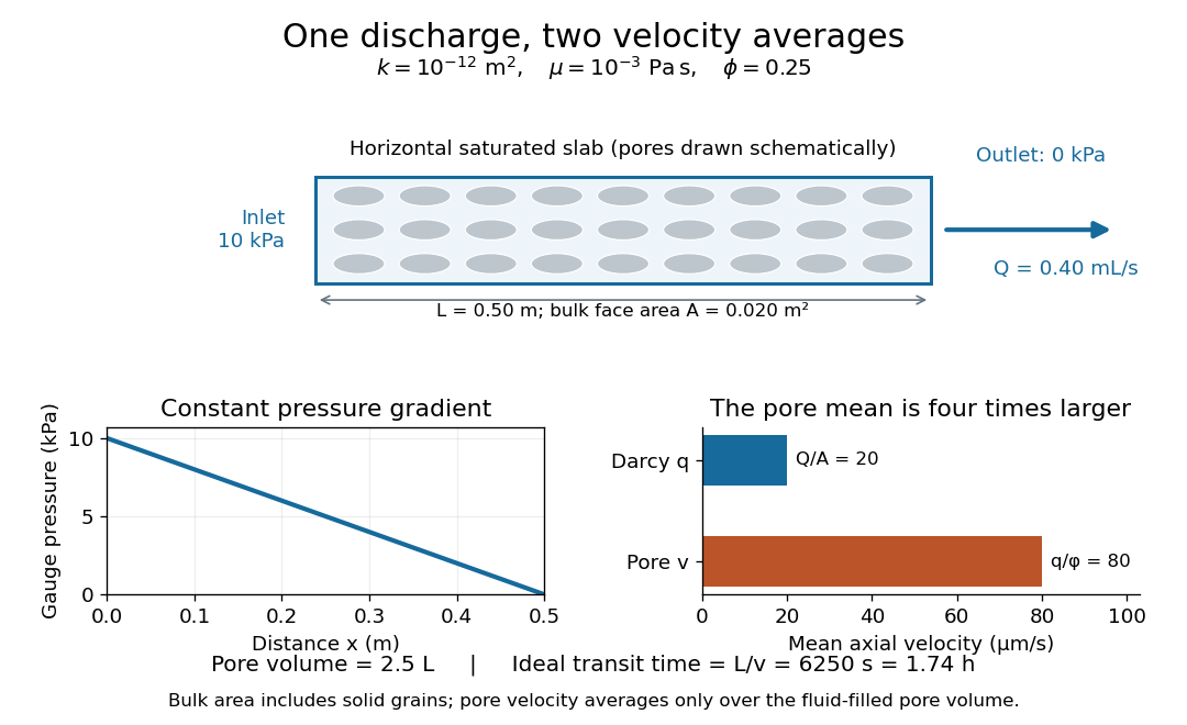
The same discharge gives different Darcy and pore velocities
. Details. Regenerate the diagram by running
python ../darcy-flux-and-pore-velocity.py from _media; it writes its PNG into the current directory.Hydraulic conductivity is the coefficient in , with units . Because the gradient of hydraulic head is dimensionless, hydraulic conductivity has the dimensions of velocity, but it is not the actual Darcy velocity unless the driving gradient has magnitude one. Intrinsic permeability of a porous medium has units and describes pore geometry; hydraulic conductivity also depends on mass density, dynamic viscosity and gravitational acceleration.[ref]
For , , and , hydraulic conductivity is . Doubling dynamic viscosity while keeping pore geometry, mass density and gravitational acceleration fixed halves hydraulic conductivity without changing intrinsic permeability of a porous medium. Thus a value quoted as a material's hydraulic conductivity needs its fluid conditions.
Hydraulic head is the sum of elevation and pressure head, measured in metres relative to a chosen height datum. For constant mass density and gravitational acceleration magnitude , the pressure head is the height of a column of the same fluid supported by fluid pressure . A water-filled open measuring tube records hydraulic head as the elevation of its water level when is gauge fluid pressure. Changing the common pressure reference or height datum adds a constant to hydraulic head and leaves its driving gradient unchanged.
For water with and , a point at with gauge fluid pressure has . A second point at with gauge fluid pressure also has : these values are compatible with a stationary column under hydrostatic pressure. It is a difference in hydraulic head, rather than a difference in fluid pressure alone, that drives saturated Darcy flow. This form uses constant mass density; one cannot generally pull spatially varying through the gradient.[ref]
For and , the identity gives the displayed reduction, since taking a th power equals substitution in characteristic . The reduction of is squarefree because it divides the separable polynomial . The Kummer-Dedekind theorem therefore gives ramification index of a prime ideal in the cyclotomic field. In particular, a conductor factor occurring only to the first power has index one and creates no ramification by itself.
Fix finitely many prescribed cyclotomic classes for pairwise differences. Such patterns are realized in every sufficiently large compatible finite field. For already chosen coordinates, let count extensions with prescribed classes for . Averaging over all gives and, from the uniform two-class intersection estimate, . The Chebyshev inequality makes the fraction with tend to zero. Inductively each fixed pattern on coordinates occupies a positive proportion of all tuples, so some positive proportion have many extensions. This proves the pattern-existence claim without an unproved greedy-extension assumption.
Pinned article: Introduction to the OurBigBook Project
Welcome to the OurBigBook Project! Our goal is to create the perfect publishing platform for STEM subjects, and get university-level students to write the best free STEM tutorials ever.
Everyone is welcome to create an account and play with the site: ourbigbook.com/go/register. We belive that students themselves can write amazing tutorials, but teachers are welcome too. You can write about anything you want, it doesn't have to be STEM or even educational. Silly test content is very welcome and you won't be penalized in any way. Just keep it legal!
Intro to OurBigBook
. Source. We have two killer features:
- topics: topics group articles by different users with the same title, e.g. here is the topic for the "Fundamental Theorem of Calculus" ourbigbook.com/go/topic/fundamental-theorem-of-calculusArticles of different users are sorted by upvote within each article page. This feature is a bit like:
- a Wikipedia where each user can have their own version of each article
- a Q&A website like Stack Overflow, where multiple people can give their views on a given topic, and the best ones are sorted by upvote. Except you don't need to wait for someone to ask first, and any topic goes, no matter how narrow or broad
This feature makes it possible for readers to find better explanations of any topic created by other writers. And it allows writers to create an explanation in a place that readers might actually find it.
Figure 1. Screenshot of the "Derivative" topic page. View it live at: ourbigbook.com/go/topic/derivativeVideo 2. OurBigBook Web topics demo. Source. - local editing: you can store all your personal knowledge base content locally in a plaintext markup format that can be edited locally and published either:This way you can be sure that even if OurBigBook.com were to go down one day (which we have no plans to do as it is quite cheap to host!), your content will still be perfectly readable as a static site.
- to OurBigBook.com to get awesome multi-user features like topics and likes
- as HTML files to a static website, which you can host yourself for free on many external providers like GitHub Pages, and remain in full control

Figure 2. You can publish local OurBigBook lightweight markup files to either OurBigBook.com or as a static website.
Figure 3. Visual Studio Code extension installation.
Figure 5. . You can also edit articles on the Web editor without installing anything locally. Video 3. Edit locally and publish demo. Source. This shows editing OurBigBook Markup and publishing it using the Visual Studio Code extension. 
- Infinitely deep tables of contents:



All our software is open source and hosted at: github.com/ourbigbook/ourbigbook
Further documentation can be found at: docs.ourbigbook.com
Feel free to reach our to us for any help or suggestions: docs.ourbigbook.com/#contact