Topics (384k) Articles (398k) Users (410) Discussions (242) Comments (383) Files (13k) New article

Molecular diffusion is the component of material transport caused by the random thermal motion of molecules, measured relative to bulk motion of their surroundings. A diffusion coefficient is a property of a particular substance in a particular medium under specified conditions, not a universal speed of spreading. Its dependence on the solute, solvent and temperature is precisely what makes a spreading experiment informative. A random walk idealizes this motion; the Brownian motion description provides a continuous approximation over sufficiently long times. [ref]
https://ocw.mit.edu/courses/1-061-transport-processes-in-the-environment-fall-2008/8260e3e1577cd739ce85143510d9c165_lec_01.pdf. Nepf, MIT: molecular motion and diffusivity
A motivating experiment: watch dye enter a gel. Samprovalaki, Robbins and Fryer studied rhodamine 6G and methylene blue entering agar gel from two side reservoirs. A covered slab, , sat on a controlled thermal stage; the dye was brought to the same temperature. They photographed the gel every ten minutes, averaged image intensity across a strip, and fitted the changing concentration to a diffusion equation model. The cover limited evaporation and stopped dye travelling over the gel surface. Runs at , and were repeated in triplicate. The measured spatial colour change therefore supplied a quantitative transport test, rather than merely showing that dye eventually spreads. Changing lighting also changes image intensity, so the optical response had to be checked. Importantly for interpretation, their constant-diffusion coefficient fit was imperfect and the gel coefficient is an effective transport coefficient, not automatically the value in free water. [ref]
A finite-pulse version to test width growth. The following is a proposed teaching variant, not that paper's apparatus or a report of measurements. Make a long, narrow, transparent gel channel of uniform cross-section. Join a thin dyed gel band between two undyed lengths of the same gel, with good contact and no air gaps; the dye should initially fill the cross-section so the dominant concentration variation is along the channel coordinate . After assembly, keep the covered channel horizontal at uniform temperature, away from vibration. The dye is a finite initial pulse: no reservoir supplies more dye. Choose a dye whose image response can be calibrated and whose interaction with the gel is small enough for an approximately constant diffusion coefficient to be plausible.
Photograph the whole pulse at recorded times with fixed lighting, focus and exposure, including a length scale. Use uniformly dyed standards of the same gel thickness and a blank gel to convert image intensity to concentration ; do not assume raw brightness is proportional to concentration. Average across the channel width and examine several parallel strips to check the one-dimensional approximation. Measure the initial profile instead of treating the band as infinitely thin. For a finite pulse with negligible end effects, define its spatial integral , centre and width byHere is the variance of the normalized profile , and is its standard deviation. If is measured in , then has units ; multiplying by the channel cross-section gives the total amount of substance. For the unbounded one-dimensional diffusion equation with constant , conserved , finite variance and sufficiently decaying tails,Thus plot width squared against time: its slope determines the diffusion coefficient, while its intercept includes the finite starting width. This moment law holds even for a non-Gaussian distribution initially; it follows by applying integration by parts twice to the diffusion equation. [ref]
https://ocw.mit.edu/courses/1-061-transport-processes-in-the-environment-fall-2008/68b0a4a664246168ee639298b39384b1_lec_03.pdf. Nepf, MIT: profile moments and estimating diffusivity from variance growth
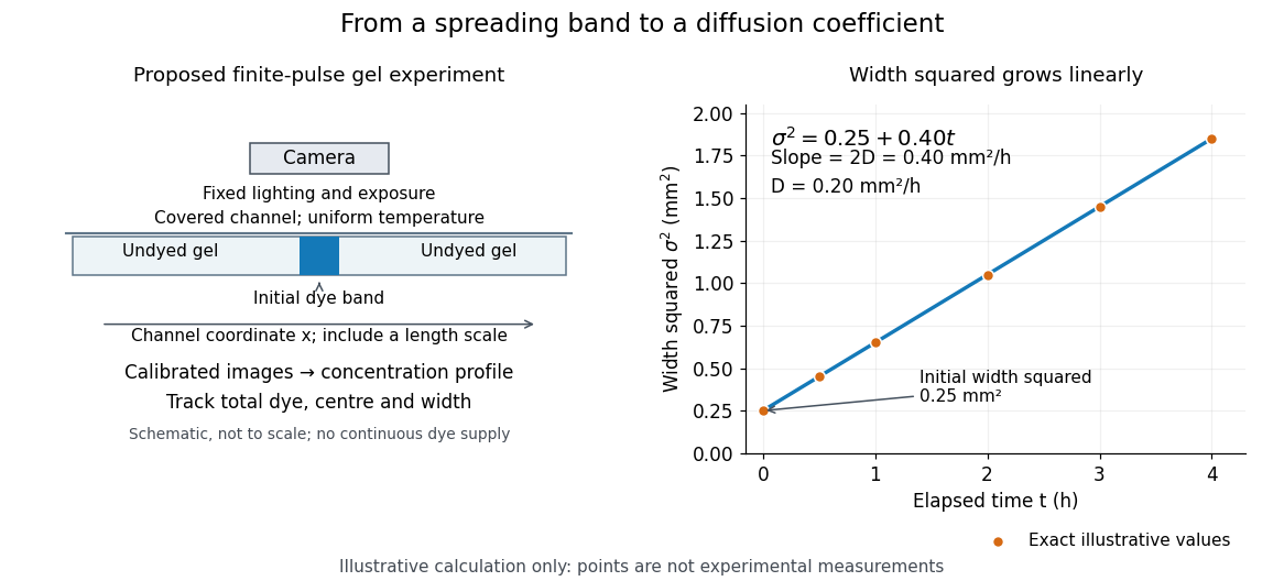
Measuring molecular diffusion from the growth of width squared
. Original schematic of the proposed finite-pulse gel experiment, with an illustrative calculation rather than measured data. A camera records the broadening band. The plotted points are exact samples of with in and in hours; the slope gives the chosen . The schematic is not to scale and is not a reproduction of the published apparatus. Details.For the particularly readable case of an initially Gaussian distribution centred at zero, uniform advection at speed and constant diffusion coefficient give the one-dimensional concentration profileIts centre moves as and its variance grows as . Our illustrative choice and gives widths , and at zero, one and four hours. These are calculated values, not a measured dye coefficient. Once dominates the initial variance, width grows as : four times the elapsed time gives approximately twice the width. A rectangular starting band will not immediately have a Gaussian distribution, although the same width-squared law still applies under the stated assumptions.
Controls and limits of the interpretation. In the proposed experiment, check that stays constant and that the centre remains stationary while the width increases. Include a blank and a uniformly dyed gel photographed over the same period: an apparent signal change there exposes lighting drift, dye fading or evaporation. Repeat with a lower starting dye concentration and a second initial width; agreement of the slopes is a check on constant and on preparation effects. Keep the pulse far from the channel ends and record its faint tails: truncation and background errors can strongly bias a variance. Poor contact, dye binding, chemical reactions or transport in a liquid film can invalidate the simple model. A gel suppresses bulk liquid motion, but its inferred diffusivity need not equal that in the pure solvent. A stationary centre alone does not exclude symmetric flows, and linear width-squared growth alone does not prove a molecular mechanism: turbulence can also produce an effective diffusive description. These are reasons to combine the profile test with the controlled setup.
In a cyclic group with generator , participants with secret exponents can exchange tokens around a ring. Token starts at and is successively exponentiated by its next recipients before being sent to the final recipient, whose exponent is the only one missing. That recipient completes the exponentiation locally. Each token makes transmissions, and everyone obtains . Thus transmitted group elements suffice. As with two-party Diffie-Hellman key exchange, authentication is needed.
For a differential three-form with on an oriented eleven-dimensional manifold, varying with fixed metric gives up to a boundary term. Indeed , so the two differentiated factors and the differentiated factor contribute equally. The shift changes the density by , preserving the field equation.
For , differentiability at means that the difference quotient has a finite two-sided limit of a function. For , require derivatives through order throughout some open neighbourhood of , and require the final difference quotientto exist as a finite real number. The last derivative need not exist elsewhere or be continuous at . In particular, existence of by itself does not justify taking a second derivative: the function must first be defined in a neighbourhood of .
At a point with , factor the difference of squares and divide by to show that differentiability of is equivalent to that of . At a zero of , its square has a local minimum; if differentiable, its derivative must vanish. The difference quotient then vanishes exactly when , equivalently . For example, with is not differentiable at zero, but its square is.
If all partial derivatives exist near a point and are continuous there, successive coordinate increments and the one-variable mean value theorem express as with . Subtracting the displayed linear map leaves , proving Fréchet differentiability. In two dimensions the absolute remainder is at most for small enough increments.
The function for , extended by , is differentiable everywhere. At zero its derivative is zero by the difference quotient, while away from zero is unbounded near zero. Differentiability of a function is therefore weaker than continuity of its derivative.
Set . The difference quotient has Euclidean norm , so . For , differentiation gives . Thus this differentiable curve has a derivative discontinuous at zero, despite each scalar component satisfying the usual one-dimensional derivative properties.
Put , take odd , and let be the index- multiplicative subgroup. If a -set has its unordered pair differences in distinct -cosets, choose containing exactly one element from each pair . Then is a difference family for a Steiner 2-design. Indeed one unordered pair supplies each coset, and its two difference orientations multiplied by cover that coset once. Translations yield a - Steiner system. The cyclotomic pattern extension by a second-moment bound supplies suitable for all sufficiently large in this progression.
Characterize the instrument and fixture before inferring permittivity: use the prescribed open and short measurements to compensate residual parallel response and series electrical impedance, and check a known reference capacitor or the required load standard. Keep cables and electrode geometry reproducible. An open fixture measurement is distinct from the empty-gap reference capacitor; blindly subtracting its entire capacitance would remove the desired reference signal. Compensation cannot determine an incorrectly measured specimen thickness or eliminate all specimen-dependent fringing field of a capacitor errors. [ref].
The dimensionless quantity relating induced electric polarization to the internal electric field through in the static scalar model. It describes the material contribution; relative permittivity includes the vacuum term as well, . Zero electric susceptibility gives , not zero permittivity.
The scalar assumes a local response with linearity and isotropy, settled electric polarization, fixed material conditions, and no residual electric polarization at zero electric field. It relates to the averaged total internal electric field, which already includes the field of the bound electric charges. It does not relate to the field the external electrodes would produce in vacuum. The distinction is essential for a self-consistent calculation.[ref]
Polarization. equations (807)–(812): total field, displacement, linear susceptibility and relative dielectric constant
Substitute the scalar relation into the definition of electric displacement field:Comparison with proves and . Both and have units , so is a dimensionless quantity. In a stipulated static model with , : at a prescribed internal electric field, the material contribution is twice . This is a hypothetical response, not a measured material constant. The electric susceptibility is a convenient bridge from microscopic dielectric polarization to a macroscopic capacitance measurement, but it is not a measure of electrical conductivity.
The image of the diagonal map in . For a manifold, the diagonal subset is an embedded submanifold diffeomorphic to .
If the input qubit of the Deutsch algorithm acquires conditional environment states with overlap between its two Hadamard gates, its fixed zero-for-constant, one-for-balanced rule succeeds with probability . A known phase can be compensated before the last Hadamard gate, raising the success probability to . An orthogonal pair of environment states gives and destroys all information in the input qubit about the answer; unit overlap modulus preserves coherence up to a known phase.
For smooth fields into with nonnegative differentiable potential and finite energy, Derrick scaling in two spatial dimensions forces the potential integral to vanish. Thus the field takes values where and , so its static field equation makes every component harmonic. Each first derivative is an entire harmonic function in L2 space; the mean-value inequality on arbitrarily large balls forces it to vanish. Hence the field is constant. The scale identity alone does not exclude a pure-gradient model; this additional argument uses the flat unconstrained target. Curved-target harmonic maps, for example the O3 nonlinear sigma model, can instead have finite-energy nonconstant solutions.
The category is obtained from bounded below cochain complexes of sheaves by passing to cochain-homotopy classes of maps and then inverting quasi-isomorphisms. It can equally be modeled by injective resolutions. The cohomology-sheaf functors descend to this localization, and an object is zero exactly when all its cohomology sheaves vanish.
A bounded complex is constructible for a given stratification when each of its cohomology sheaves restricts to a finite-rank local system on every stratum. Constructibility concerns cohomology sheaves, not an arbitrary choice of resolution.
On bounded constructible complexes over locally compact stratified spaces, Verdier duality is , where is the dualizing complex. For an oriented real -manifold, . Proper direct image commutes with this duality, and . These properties exchange stalk support conditions with costalk conditions.
A ghost is a morphism inducing zero on every cohomology sheaf, but it need not itself be zero. For the equator and complement , the connecting morphism is a ghost. Its source and target have cohomology sheaves in different degrees, but its induced map is nonzero, proving that the derived morphism is nonzero.
For a perfect fluid with , in Newtonian gauge in cosmology the density perturbation on fluid-comoving slices is the displayed combination of the fractional density perturbation and velocity potential. The Einstein energy and momentum constraints combine into when scalar anisotropic stress vanishes. This gives a relativistic Poisson constraint valid beyond the subhorizon limit.
Revealed preference infers rankings from choices: a chosen bundle is directly revealed at least as desirable as any bundle affordable in the same budget. Indirect comparisons use chains of such observations.
Pinned article: Introduction to the OurBigBook Project
Welcome to the OurBigBook Project! Our goal is to create the perfect publishing platform for STEM subjects, and get university-level students to write the best free STEM tutorials ever.
Everyone is welcome to create an account and play with the site: ourbigbook.com/go/register. We belive that students themselves can write amazing tutorials, but teachers are welcome too. You can write about anything you want, it doesn't have to be STEM or even educational. Silly test content is very welcome and you won't be penalized in any way. Just keep it legal!
Intro to OurBigBook
. Source. We have two killer features:
- topics: topics group articles by different users with the same title, e.g. here is the topic for the "Fundamental Theorem of Calculus" ourbigbook.com/go/topic/fundamental-theorem-of-calculusArticles of different users are sorted by upvote within each article page. This feature is a bit like:
- a Wikipedia where each user can have their own version of each article
- a Q&A website like Stack Overflow, where multiple people can give their views on a given topic, and the best ones are sorted by upvote. Except you don't need to wait for someone to ask first, and any topic goes, no matter how narrow or broad
This feature makes it possible for readers to find better explanations of any topic created by other writers. And it allows writers to create an explanation in a place that readers might actually find it.
Figure 1. Screenshot of the "Derivative" topic page. View it live at: ourbigbook.com/go/topic/derivativeVideo 2. OurBigBook Web topics demo. Source. - local editing: you can store all your personal knowledge base content locally in a plaintext markup format that can be edited locally and published either:This way you can be sure that even if OurBigBook.com were to go down one day (which we have no plans to do as it is quite cheap to host!), your content will still be perfectly readable as a static site.
- to OurBigBook.com to get awesome multi-user features like topics and likes
- as HTML files to a static website, which you can host yourself for free on many external providers like GitHub Pages, and remain in full control

Figure 2. You can publish local OurBigBook lightweight markup files to either OurBigBook.com or as a static website.
Figure 3. Visual Studio Code extension installation.
Figure 5. . You can also edit articles on the Web editor without installing anything locally. Video 3. Edit locally and publish demo. Source. This shows editing OurBigBook Markup and publishing it using the Visual Studio Code extension. 
- Infinitely deep tables of contents:



All our software is open source and hosted at: github.com/ourbigbook/ourbigbook
Further documentation can be found at: docs.ourbigbook.com
Feel free to reach our to us for any help or suggestions: docs.ourbigbook.com/#contact