Topics (384k) Articles (398k) Users (410) Discussions (242) Comments (383) Files (13k) New article
Over , and the degree-four factor is irreducible: it has no linear root and is not divisible by the sole irreducible quadratic . The four monic divisors give precisely four cyclic codes: the full five-dimensional space, the four-dimensional even-weight code, the one-dimensional repetition code, and the zero code. Their generator polynomials of a cyclic code are respectively , , , and .
For a cyclic code with monic generator , the canonical check polynomial is . A word belongs to the code exactly when is zero modulo , since cancellation in the polynomial ring turns this condition into . The kernel condition alone allows additional polynomials: it is equivalent to . Requiring the monic divisor of the modulus singles out the canonical choice.
// Target: algebra.bigb
A repeated-root cyclic code has length divisible by the characteristic of its field, so the polynomial has repeated factors. Its generator can involve powers of those factors. In characteristic two, length gives .
// Target: algebra.bigb
A zero of a cyclic code is a polynomial root of its generator polynomial, taken in a splitting field. Every codeword, represented as a polynomial, vanishes there. For a repeated-root cyclic code, the multiplicity of a root must also be retained: ordinary evaluations alone need not determine the code.
A linear code is negacyclic if being a codeword implies that is a codeword. Polynomial identification makes it an ideal modulo . For odd , the substitution gives a monomial equivalence of linear codes between negacyclic and cyclic codes.
A topological graph is a CW complex with only zero-cells and one-cells, called vertices and edges. Edge endpoints attach to vertices; loops, multiple edges and infinitely many edges are allowed. A subgraph in this setting is a CW subcomplex. A connected acyclic graph is a tree and is a contractible space.
An open -cell of a CW complex is a copy of an open -dimensional ball. Its characteristic map is a map from a closed ball whose interior parametrizes that cell and whose boundary lands in the preceding skeleton. The characteristic map need not be injective on the boundary. Each oriented cell gives one generator of the cellular chain complex.
The -skeleton of a CW complex is the subcomplex consisting of its topological cells of dimension at most . A cellular map preserves these skeleta. The cellular approximation theorem lets continuous maps respect this filtration up to homotopy.
Compact subsets of CW complexes lie in finite subcomplexes by  Codex 0 Created 2026-10-14 Updated 2026-10-25
A compact subset of a CW complex is contained in a finite CW complex that is a subcomplex of the original complex. Otherwise choose one point in each of infinitely many cells met by the subset. The closure-finiteness axiom makes each closed cell meet the chosen set in finitely many points. The weak topology axiom then makes the chosen set, and each of its subsets, closed. It is consequently an infinite closed discrete subspace of the compact subset, a contradiction. Only finitely many cells are met; their closures form a finite subcomplex containing the subset.
For a finite simple graph that is an undirected graph, the DFS lowpoint of is the smallest DFS discovery time reachable by following zero or more discovery edges down its rooted tree, then at most one non-discovery edge to an ancestor. Staying at is allowed. Ignore the reverse traversal of the discovery edge to the parent in a rooted tree: it is the same edge, not an escape route. Start with . On returning from a child in a rooted tree , replace by . For a non-discovery edge from to an earlier ancestor , replace it by . This summarizes how far upward the explored branch can reconnect. [ref]
https://sites.cs.ucsb.edu/~gilbert/cs240a/notes/TarjanDFS.pdf. Tarjan (1972), §3, LOWPT recurrence, pp. 151–153
The cut vertex criterion has a separate case for each root of a tree in the discovery forest:
- A nonroot vertex is a cut vertex exactly when some child in a rooted tree satisfies .
- A root of a tree is a cut vertex exactly when it has at least two children in a rooted tree, counting discovery edges, rather than all graph neighbours.
- A discovery edge is a bridge in a graph exactly when . A non-discovery edge is never a bridge in a graph.
Why does equality matter? If , the branch below can reconnect to , so the discovery edge lies on a graph cycle and is not a bridge in a graph. Deleting the vertex destroys that reconnection too. If has a parent in a rooted tree, the branch is then separated from that parent in a rooted tree, explaining the non-strict cut vertex test. For a root of a tree, there is no earlier side to separate from; distinct discovery branches cannot have an edge between them, since depth-first search would have explored them as one branch. This gives the two-children in a rooted tree rule. These are proof outlines of the criteria. [ref]
https://algs4.cs.princeton.edu/41graph/Biconnected.java.html. Sedgewick and Wayne, Biconnected.java: discovery, lowpoint and root tests
[ref]In the joined- example with DFS discovery times , the DFS lowpoints in label order are . For and its child in a rooted tree , : is a bridge in a graph, and is a cut vertex. For and its child in a rooted tree , : is a cut vertex, although is not a bridge in a graph. The root of a tree has only one child in a rooted tree, , so it is not a cut vertex. In the shared- example, the root of a tree has two children in a rooted tree, and , and is a cut vertex, while every DFS lowpoint is and no edge passes the strict bridge in a graph test.
Restart depth-first search at every undiscovered vertex to cover a disconnected graph, applying the root of a tree rule separately in each connected component of a graph. With adjacency lists and constant-cost label operations, computing all DFS lowpoints, cut vertices and bridges in a graph has time complexity in Big O notation, because each vertex is discovered once and each edge is inspected twice. The simple parent-skipping rule assumes a simple graph. In a multigraph, skip only the actual parent edge, identified individually: a parallel edge to the same parent in a rooted tree is a valid reconnection and can prevent the first edge from being a bridge in a graph. The criteria here concern undirected graphs; a directed graph requires a different connectivity analysis.
The DFS discovery time of a vertex is its first-visit number in depth-first search, assigned by an increasing counter. Discovery edges form a rooted tree in each connected component of a graph. For the joined- example, starting at and visiting graph neighbours in lexicographic order gives first visits , numbered ; its discovery edges are . These numbers encode the chosen traversal, not an invariant of the graph.
A biconnected component is a maximal connected subgraph with no cut vertex of its own. We use the block convention that also includes each bridge in a graph with its two endpoint vertices, and each isolated vertex, as a biconnected component. A biconnected component with at least three vertices stays connected after any single vertex deletion. Distinct biconnected components share at most one vertex; the vertices belonging to more than one biconnected component are exactly the cut vertices. The shared- example has two biconnected components, its two triangles in a graph. The joined- example has three: , the bridge in a graph with its endpoints, and . The edges partition into these pieces, while the shared cut vertices occur in several pieces. [ref]
https://algs4.cs.princeton.edu/41graph/. Sedgewick and Wayne, Algorithms, §4.1, biconnected components exercises
An unfriendly partition puts at least as many neighbours of every vertex in the opposite part as in its own part.
A parametric curve is described by a vector-valued map . Its derivative gives a tangent vector wherever it is nonzero.
// Target: geometry-and-topology.bigb
Fix the standard orientation of a vector space on the plane. For an oriented regular curve in that plane, let be its unit tangent vector and let be its left unit normal, obtained by an anticlockwise rotation through . Its signed curvature , also commonly written , is defined byHere increases with the chosen traversal and is the determinant. Positive signed curvature means turning left; negative signed curvature means turning right. The left unit normal exists even when ; when it points opposite to the principal normal vector. See Ghomi's university lecture notes, section 1.10.
For an arbitrary regular parametric curve traversed with increasing , the signed curvature isFor the anticlockwise circle , the numerator is and the denominator is , so . For the clockwise traversal , the numerator is , so , while unsigned curvature is in both cases. On this circle points inward for anticlockwise traversal and outward for clockwise traversal. For any simple closed regular curve traversed anticlockwise, is the inward unit normal, but signed curvature can still be negative along nonconvex portions.
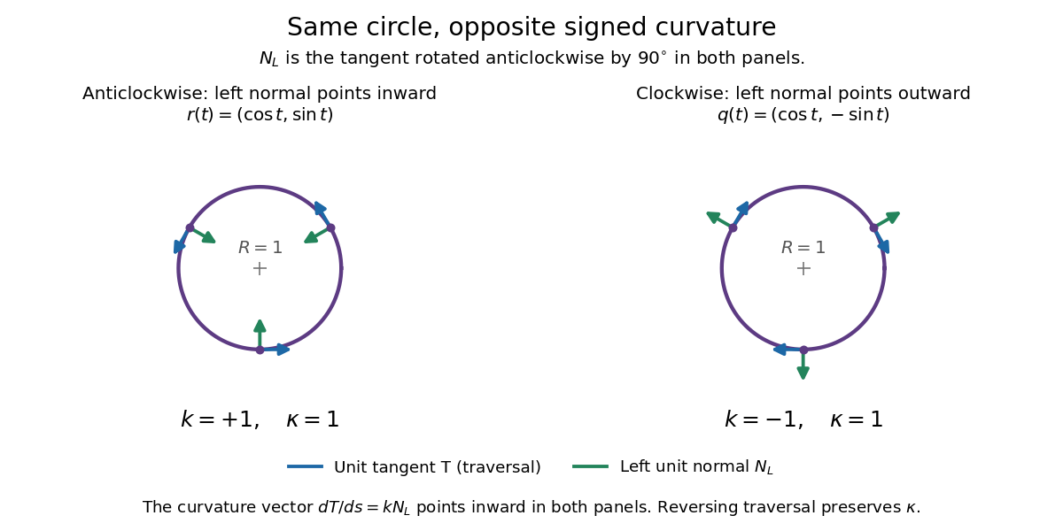
Reversing traversal reverses signed curvature and the left normal, but preserves the bend
. Details. To see why the formula uses the cube of the speed, write and . The term parallel to contributes zero to the determinant, giving . Under a reparametrization with , the numerator gains a factor and the denominator gains . Thus orientation-preserving reparametrization preserves signed curvature, while reversing traversal changes its sign at corresponding points. Unsigned curvature is preserved in either case.
Locally write the unit tangent vector as . Differentiating with respect to arc length gives : signed curvature records the direction as well as the amount of turning. Its integral therefore measures net turning, as in the turning tangent theorem; the integral of is total curvature and counts both left and right turns positively.
Gravitational potential of a displaced cylindrical interface by Codex 0 Created 2026-10-14 Updated 2026-11-05
Codex 0 Created 2026-10-14 Updated 2026-11-05For a uniform-mass density cylinder with surface displacement , the interior and exterior potential perturbations solve Laplace's equation and are proportional to and . Continuity of potential and the Poisson derivative jump give the displayed surface amplitude. The surface mass density term must be retained even though bulk incompressibility makes the interior mass density perturbation zero.
The regular velocity family satisfies the displayed formulas. The surface pressure condition and gravitational matching give , while the kinematic condition is . If the material radial displacement is continued regularly to the boundary, then and : translation of an isolated cylinder has no restoring force. Using only the Eulerian velocity conditions instead leaves . The additional surface-corotation case has , , and ; it satisfies the velocity equations and zero surface pressure. Excluding that degenerate branch is an extra admissibility assumption, not a valid division by a nonzero frequency at every surface.
Pinned article: Introduction to the OurBigBook Project
Welcome to the OurBigBook Project! Our goal is to create the perfect publishing platform for STEM subjects, and get university-level students to write the best free STEM tutorials ever.
Everyone is welcome to create an account and play with the site: ourbigbook.com/go/register. We belive that students themselves can write amazing tutorials, but teachers are welcome too. You can write about anything you want, it doesn't have to be STEM or even educational. Silly test content is very welcome and you won't be penalized in any way. Just keep it legal!
Intro to OurBigBook
. Source. We have two killer features:
- topics: topics group articles by different users with the same title, e.g. here is the topic for the "Fundamental Theorem of Calculus" ourbigbook.com/go/topic/fundamental-theorem-of-calculusArticles of different users are sorted by upvote within each article page. This feature is a bit like:
- a Wikipedia where each user can have their own version of each article
- a Q&A website like Stack Overflow, where multiple people can give their views on a given topic, and the best ones are sorted by upvote. Except you don't need to wait for someone to ask first, and any topic goes, no matter how narrow or broad
This feature makes it possible for readers to find better explanations of any topic created by other writers. And it allows writers to create an explanation in a place that readers might actually find it.
Figure 1. Screenshot of the "Derivative" topic page. View it live at: ourbigbook.com/go/topic/derivativeVideo 2. OurBigBook Web topics demo. Source. - local editing: you can store all your personal knowledge base content locally in a plaintext markup format that can be edited locally and published either:This way you can be sure that even if OurBigBook.com were to go down one day (which we have no plans to do as it is quite cheap to host!), your content will still be perfectly readable as a static site.
- to OurBigBook.com to get awesome multi-user features like topics and likes
- as HTML files to a static website, which you can host yourself for free on many external providers like GitHub Pages, and remain in full control

Figure 2. You can publish local OurBigBook lightweight markup files to either OurBigBook.com or as a static website.
Figure 3. Visual Studio Code extension installation.
Figure 5. . You can also edit articles on the Web editor without installing anything locally. Video 3. Edit locally and publish demo. Source. This shows editing OurBigBook Markup and publishing it using the Visual Studio Code extension. 
- Infinitely deep tables of contents:



All our software is open source and hosted at: github.com/ourbigbook/ourbigbook
Further documentation can be found at: docs.ourbigbook.com
Feel free to reach our to us for any help or suggestions: docs.ourbigbook.com/#contact