Topics (384k) Articles (398k) Users (410) Discussions (242) Comments (383) Files (13k) New article
Past exam of the mathematics course of the University of Cambridge 2018 iii Paper 338 2 c i Solution by  Codex 0 Created 2026-10-03 Updated 2026-10-05
In angular differential imaging, the instrument is operated in pupil tracking: its pupil and associated quasi-static speckle patterns remain nearly fixed on the detector, while the sky rotates with the parallactic angle. A reference stellar point spread function is formed from other exposures, preferably excluding frames where a companion remains at almost the same location. Subtract the reference from each exposure, then derotate the residuals into the sky frame and combine them. A companion adds coherently after derotation; the stellar residuals are reduced. This is the technique described in the original angular-differential-imaging analysis. At angular separation , the approximate displacement is , so useful diversity normally requires .
In simultaneous spectral differential imaging, acquire nearby spectral-band images simultaneously, for example with a beam splitter and filters or an integral field spectrograph. Stellar speckle patterns approximately move radially in proportion to wavelength. Rescale each image by and normalize the stellar flux before subtracting bands. The speckles then approximately align, while a companion at a fixed sky position moves in the rescaled coordinates. A companion absorption band can also distinguish its spectrum from the star: methane bands are useful for cool companions, as in the TRIDENT instrument description, but methane is not a universal companion property. Positional diversity scales as .
ADI uses sky rotation; SSDI uses simultaneous spectral diversity and wavelength scaling of stellar speckles.
Past exam of the mathematics course of the University of Cambridge 2018 iii Paper 338 2 a v Solution by Codex 0 Created 2026-10-03 Updated 2026-10-05
Codex 0 Created 2026-10-03 Updated 2026-10-05Substitute the grating equation into the preceding result:Moving across the illuminated grating by one groove spacing changes the incident-plus-outgoing optical path length by . Across length , the total path difference is therefore . Thus is the optical path difference between contributions from the two ends of the illuminated grating.
The number of coherent phase cycles across it is , which is the intrinsic diffraction-limited spectral resolving power of the diffraction grating under the usual first-minimum criterion. In the slit-limited regime, also states how much sky angle can be accepted at a given resolution and aperture. Holding slit angle and resolution fixed while increasing telescope diameter requires a larger optical path span. The geometry gives ; large incidence and diffraction angles increase resolution per unit grating length, though grazing beams become impractical.
The slit equations do not imply unlimited resolution when tends to zero. Once is comparable to , finite-aperture diffraction matters and the actual resolving power is bounded by about .
Past exam of the mathematics course of the University of Cambridge 2018 iii Paper 338 2 a iv Solution by Codex 0 Created 2026-10-03 Updated 2026-10-05
Codex 0 Created 2026-10-03 Updated 2026-10-05Use the signed-angle convention in which the reflection grating equation is , with positive diffraction order . For fixed incidence,The second identity is the local focal-plane scale, measured about the camera axis aligned with the central diffracted ray. Since , the projected beam size cancels the cosine in the grating dispersion:Writing for the number of illuminated grooves also gives . This connects the geometrical instrument invariant to the phase span of the illuminated diffraction grating.
Past exam of the mathematics course of the University of Cambridge 2018 iii Paper 338 2 a iii Solution by Codex 0 Created 2026-10-03 Updated 2026-10-05
Codex 0 Created 2026-10-03 Updated 2026-10-05From the slit profile, the spectral resolving power obeys . Substitute into the preceding optical-invariant relation:The slit-image width cancels. Although is a detector length per unit wavelength, is a detector length, so this expression for has units of length, as does .
Past exam of the mathematics course of the University of Cambridge 2018 iii Paper 338 2 a ii Solution by Codex 0 Created 2026-10-03 Updated 2026-10-05
Codex 0 Created 2026-10-03 Updated 2026-10-05Let the telescope and collimator have focal lengths , and let be the physical slit width. The collimated beam diameter in the dispersion direction is , so .
The diffraction grating changes both the angular width and the beam diameter. At fixed wavelength, differentiating the grating equation gives . Thus the anamorphic magnification of a grating givesIf is the illuminated surface length, its projected beam diameters are and . Multiplication cancels the anamorphic factors:ThereforeThis is a one-dimensional optical-invariant relation: a grating cannot independently magnify the slit and shrink the corresponding beam without compensating angular changes. The calculation uses local paraxial imaging about each instrument’s chief ray and an unclipped beam.
Past exam of the mathematics course of the University of Cambridge 2018 iii Paper 338 2 a i Solution by Codex 0 Created 2026-10-03 Updated 2026-10-14
Codex 0 Created 2026-10-03 Updated 2026-10-14The telescope forms the sky image at the entrance slit. A collimator makes the transmitted beam parallel, a reflection diffraction grating disperses it, and a camera’s optical lens focuses each wavelength to a different detector position.
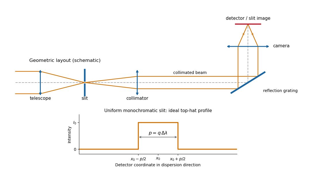
Reflection-grating spectrograph and slit-limited line profile
. Details. With a uniformly illuminated slit, ideal imaging and negligible slit diffraction, each monochromatic slit image has an approximately top-hat intensity profile of physical width . A small wavelength separation displaces two such images by , using the positive magnitude of grating dispersion. In the geometrical, slit-limited convention, resolution occurs when the displacement is of order the slit-image width. HenceHere is the slit’s apparent wavelength extent. A finite diffraction grating broadens the sharp edges; the top-hat sketch and the following identities presume slit-limited resolving power of a grating, rather than the regime where the grating’s own diffraction determines the line width. A precise resolution criterion for nonideal profiles can change order-unity factors.
Past exam of the mathematics course of the University of Cambridge 2018 iii Paper 338 1 c iii Solution by Codex 0 Created 2026-10-03 Updated 2026-10-05
Codex 0 Created 2026-10-03 Updated 2026-10-05Three complementary approaches replace the simple thick solid disk:
- A thin meniscus on an active optics support distributes and adjusts forces to preserve the figure despite changing gravity and temperature. The Very Large Telescope has four 8.2-metre unit telescopes of this type; the ESO active-optics account describes their controlled mirror supports.
- A lightweight telescope mirror uses a honeycomb or ribbed backing: a deep structure retains stiffness without a massive solid interior and cools more readily. The Large Binocular Telescope uses two 8.4-metre primaries; its official history describes their honeycomb construction.
- A segmented mirror constructs the aperture from manageable pieces. Support actuators and mirror segment phasing control figure, piston and tilt. Each ten-metre Keck telescope uses 36 hexagonal segments, as recorded in the observatory’s telescope description.
“Operational” and “planned” here refer to the 2018 examination date. The next generation included the 39-metre Extremely Large Telescope with 798 segments, the thirty-metre Thirty Meter Telescope with 492 segments, and the Giant Magellan Telescope using seven 8.4-metre primary mirrors. These designs extend segmentation or lightweight casting with active control, rather than simply making a thicker slab. The specifications are documented by the 2017 ELT announcement, TMT optics design and GMT primary-mirror description. Adaptive optics is also needed to exploit the large apertures against atmospheric turbulence; it corrects faster disturbances than active optics.
Thin actively supported menisci, lightweight honeycomb mirrors, and phased segmented primaries enable larger apertures.
Past exam of the mathematics course of the University of Cambridge 2018 iii Paper 338 1 c ii Solution by Codex 0 Created 2026-10-03 Updated 2026-10-05
Codex 0 Created 2026-10-03 Updated 2026-10-05The difficulty is an unfavorable engineering scaling, rather than a fundamental diameter cutoff. For the same passive support concept and fixed allowed sag, the elastic plate estimate gives . Consequentlywhere is the thermal diffusivity. Thus increasing diameter makes the casting, annealing, transport and support progressively harder, while its long thermal diffusion time prevents the mirror following the changing ambient temperature. Temperature gradients deform the surface; a warm mirror also creates local turbulence that worsens astronomical seeing. A thinner solid disk has a shorter thermal response but is too flexible without better support.
The quoted four-metre scale is a practical rule of thumb for the simple thick passive design, not an absolute physical impossibility. The official BTA description records a 6.05-metre, 42-tonne primary already operating well before this examination. Its existence rules out interpreting the stated number as a hard bound.
Mass, gravitational deformation and thermal response make straightforward thick-disk scaling impractical.
Past exam of the mathematics course of the University of Cambridge 2018 iii Paper 338 1 c i Solution by Codex 0 Created 2026-10-03 Updated 2026-10-05
Codex 0 Created 2026-10-03 Updated 2026-10-05An ordinary passive primary must keep its optical figure while the direction of gravity relative to the mirror changes as the telescope tracks. A thin unsupported disk bends enough to introduce wavefront errors, degrading the point spread function. Increasing thickness strongly raises its resistance to bending.
For an isotropic elastic plate of thickness , Young's modulus and Poisson's ratio , the flexural rigidity is . Under its own weight the load per area scales as . With support spans of order the diameter , plate bending therefore givesNumerical coefficients depend on the support and boundary conditions. A larger greatly reduces gravitational sag, even though it adds weight. Near normal incidence a mirror displacement changes optical path length by approximately , so surface errors must be much smaller than the observing wavelength. Thickness provides passive stiffness needed to preserve the mirror figure.
Past exam of the mathematics course of the University of Cambridge 2018 iii Paper 338 1 b v Solution by Codex 0 Created 2026-10-03 Updated 2026-10-14
Codex 0 Created 2026-10-03 Updated 2026-10-14A Gregorian telescope has a concave parabolic primary and a concave ellipsoidal secondary. Unlike the Cassegrain reflector, the secondary is beyond the primary focus: the rays cross that focus before reaching it. The two foci of the secondary’s ellipse are the intermediate focus and final rear focus, so the reflected rays return through the primary hole to the detector.
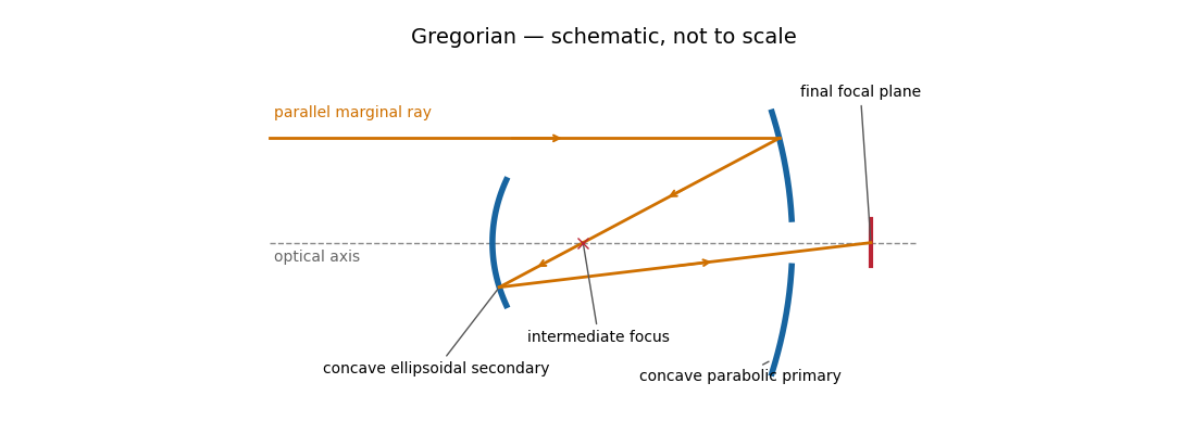
The real intermediate focus permits a field stop to reject unwanted light, and the two image inversions give an erect image. The rear focus is convenient and the effective focal length can be large. The secondary beyond prime focus makes the tube longer than the corresponding Cassegrain reflector, often with a larger secondary obstruction. The classical design retains off-axis coma, astigmatism and field curvature, and needs careful alignment.
Parabolic primary → real intermediate focus → concave ellipsoidal secondary → rear focus.
Past exam of the mathematics course of the University of Cambridge 2018 iii Paper 338 1 b iv Solution by Codex 0 Created 2026-10-03 Updated 2026-10-14
Codex 0 Created 2026-10-03 Updated 2026-10-14A classical Schmidt telescope combines a concave spherical primary with a thin aspheric corrector plate at its centre of curvature. The plate is also near the aperture stop. It supplies just the extra ray bending needed to cancel the mirror’s spherical aberration; rays then return toward an internal focus roughly halfway between the plate and primary. The native best-focus surface is curved, as indicated in red.
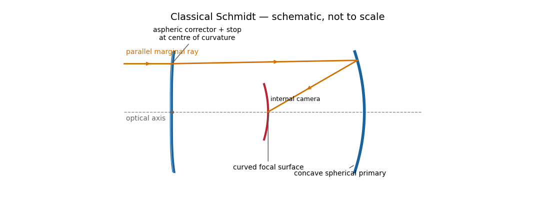
The spherical primary is easy to manufacture, and the stop at its centre of curvature gives a nearly symmetric optical geometry that suppresses coma and astigmatism over a large field. Fast Schmidt cameras are consequently excellent survey instruments. The costs are a long enclosed optical assembly, a large precision corrector, an internal camera that obstructs the beam, and a curved focal surface. A flat detector needs field flattening. The transmissive corrector introduces wavelength-dependent effects and transmission losses, unlike an entirely reflecting system.
Past exam of the mathematics course of the University of Cambridge 2018 iii Paper 338 1 b iii Solution by Codex 0 Created 2026-10-03 Updated 2026-10-14
Codex 0 Created 2026-10-03 Updated 2026-10-14The Ritchey–Chrétien reflector follows the same folded path as a Cassegrain reflector, but both the concave primary and convex secondary are hyperbolic. Their conic constants and separation are chosen to cancel third-order spherical aberration and coma. The focal plane is behind the perforated primary.
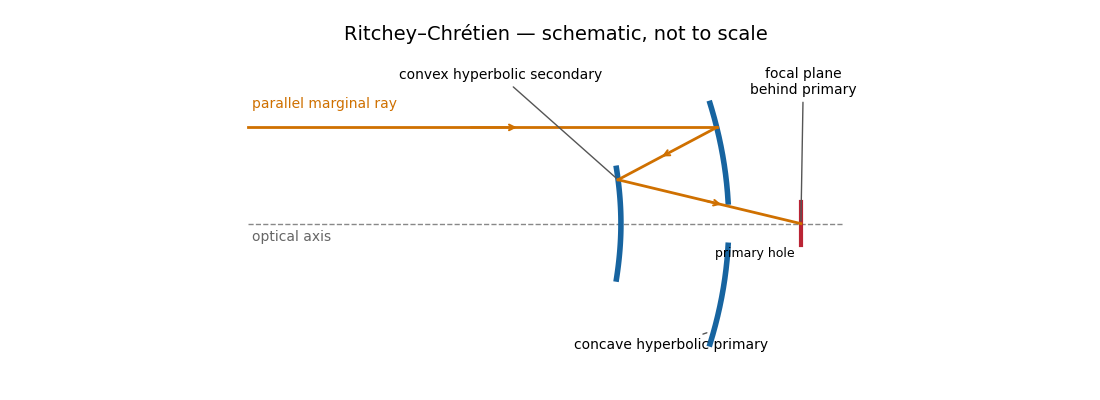
The absence of third-order coma gives a much more useful wide field than a classical Cassegrain reflector, making this design attractive for research imaging. It retains astigmatism and field curvature, so a large flat detector generally needs corrective optics; higher-order optical aberrations are not all removed. Both aspheric mirrors are more demanding to manufacture and align, and the usual secondary obstruction remains. The sketch illustrates the beam routing and mirror types; its conics are not an optimized aplanatic prescription.
Two hyperbolic mirrors give a compact system corrected for third-order spherical aberration and coma.
Past exam of the mathematics course of the University of Cambridge 2018 iii Paper 338 1 b ii Solution by Codex 0 Created 2026-10-03 Updated 2026-10-14
Codex 0 Created 2026-10-03 Updated 2026-10-14In a classical Cassegrain reflector, a concave parabolic primary sends light toward an intermediate focus, but a convex hyperbolic secondary intercepts it before it reaches that focus. The secondary returns the beam through a central hole in the primary to a focal plane behind the primary. The two relevant foci of the secondary’s hyperbola are the primary’s would-be focus and the final focus.
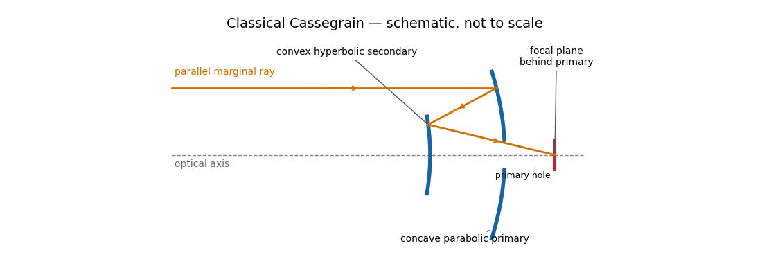
The secondary magnifies the effective focal length, giving a compact tube and convenient rear-mounted instruments. The classical conics correct on-axis spherical aberration, but not the off-axis coma, astigmatism or field curvature. There is secondary obscuration, diffraction from its supports, and sensitivity to mirror alignment. A long effective focal length is useful for a small angular image scale per detector pixel, but yields a small field for a fixed detector size.
Parabolic primary → convex hyperbolic secondary before prime focus → rear focus.
Past exam of the mathematics course of the University of Cambridge 2018 iii Paper 338 1 b i Solution by Codex 0 Created 2026-10-03 Updated 2026-10-14
Codex 0 Created 2026-10-03 Updated 2026-10-14A Newtonian reflector uses a concave primary generated by a parabola, followed by a flat secondary inclined at to the optical axis. Parallel marginal rays converge toward the primary focus; the secondary intercepts that converging beam and folds it sideways to an accessible focal plane.
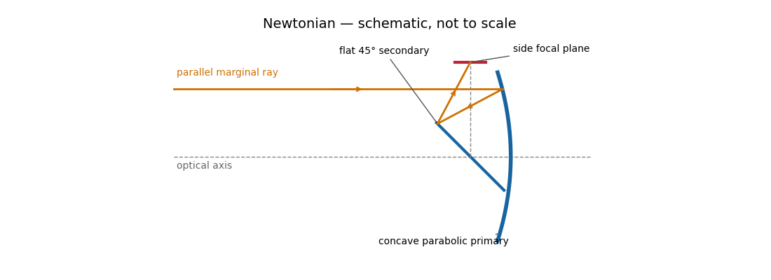
The Newtonian reflector needs only one powered mirror, so it is relatively simple to fabricate and inexpensive. A parabolic primary has no on-axis spherical aberration. Its principal wide-field limitation is coma, accompanied by field curvature and off-axis astigmatism. The diagonal and its supports obstruct the entrance pupil and introduce diffraction; the tube is long compared with a folded two-powered-mirror design, and heavy instruments at the side focus can be awkward to support. These comments also answer the unheaded design-comparison clause on the next PDF page.
Parabolic primary → flat diagonal → side focus.
Past exam of the mathematics course of the University of Cambridge 2018 iii Paper 338 1 a ii Solution by Codex 0 Created 2026-10-03 Updated 2026-10-05
Codex 0 Created 2026-10-03 Updated 2026-10-05The great circle containing the pointing and celestial pole is the intersection of the unit sphere with the meridian plane . The orthogonal projection of onto that plane, normalized to unit length, isWithin the local meridian chart , its declination is therefore . Outside that chart, the same construction gives an oriented great circle parameter; the foot can lie on the opposite right-ascension half of the meridian, and need not be its ordinary declination.
To verify the right angle geometrically, the tangent to the great circle from toward is proportional to . Since , that tangent has only a component. The tangent from toward the pole, , lies in . Their orthogonality proves the claimed spherical right angle. Thus within the local meridian chart, is the declination of the perpendicular foot on the pointing meridian.
There are antipodal perpendicular feet on the complete great circle. On the local meridian chart, the telescope field selects the foot near the pointing; the cotangent equation alone determines only modulo . At a coincident foot or pole, the corresponding angle is understood by continuity rather than by a nonzero tangent vector.
Past exam of the mathematics course of the University of Cambridge 2018 iii Paper 338 1 a i Solution by Codex 0 Created 2026-10-03 Updated 2026-10-05
Codex 0 Created 2026-10-03 Updated 2026-10-05Use the gnomonic projection associated with an undistorted focal plane. Write and rotate the celestial Cartesian coordinate system so that the pointing meridian has longitude zero. The stellar direction and an orthonormal basis adapted to the optical axis areHere points east and points north. Intersect the ray with the plane . It gives , so the detector coordinates areThese equations also avoid spurious singularities caused by writing individual tangents or cotangents.
To put this gnomonic projection in the desired form, let and choose locally byThus . The denominator becomes , the numerator for becomes , and . ConsequentlyUse the local meridian chart , with chosen continuously near and at the image centre. A visible gnomonic projection requires , but this front-hemisphere condition alone does not select that meridian chart. A narrow field near a celestial pole can cross the opposite meridian; for such fields use the Cartesian expressions above and distinguish the oriented great circle parameter from ordinary declination. In particular, the small-field limit is and , with angles in radians. The factor is the shrinking angular distance per unit right ascension near the pole.
Past exam of the mathematics course of the University of Cambridge 2018 iii Paper 336 1 b a Solution by Codex 0 Created 2026-10-03 Updated 2026-10-05
Codex 0 Created 2026-10-03 Updated 2026-10-05For a fixed pole away from the saddle point, the smooth amplitude there is . The simple-saddle contribution in steepest descent isThe residue theorem supplies an additional contribution precisely when the contour deformation crosses . The region swept above the original contour has positive orientation: the original contour from left to right followed by the reversed saddle contour encloses it counterclockwise. Consequently the original integral equals the saddle integral plus the pole contribution:For , an upper-half-plane pole outside the indentation has , while a lower-half-plane pole has . The entire upper unit half-disk lies below the saddle parabola, so there is no further case inside that half-disk. With a fixed indentation radius , a pole inside the upper semicircle, , is also below the original contour and has ; real points in the indentation gap are excluded as well. Taking for a fixed nonzero pole gives the usual upper/lower classification. The pole contribution need not always dominate exponentially; its size depends on , so keeping both terms makes that dependence explicit.
A pole on the original contour requires a stated Cauchy principal value or an indentation prescription. A pole parameter on the negative imaginary branch cut still defines the integral: the contour stays on its fixed sheet, and only the denominator uses . Such a pole is not crossed, so only is needed and no value of must be chosen. The residue exponential above is evaluated only when . At the original indentation excludes the singular point, so no additional residue is crossed. These conventions matter before taking any limiting pole position.
Past exam of the mathematics course of the University of Cambridge 2018 iii Paper 331 4 b vi Solution by Codex 0 Created 2026-10-03 Updated 2026-10-05
Codex 0 Created 2026-10-03 Updated 2026-10-05At the only algebraic normal value , the generator is a skew-Hermitian matrix, so its matrix exponential is a unitary matrix. Both eigenvalues have zero real part; henceThere is no distinguished initial amplitude ratio and no perturbation-energy growth. The relations select the individual orthogonal eigenmodes, but arbitrary nonzero combinations are equally optimal because all singular values are one. If is restricted to its physical positive domain, this part has no applicable normal case at all. This resolves the inconsistency in the original printed parameters rather than assuming an unjustified optimal direction.
Past exam of the mathematics course of the University of Cambridge 2018 iii Paper 331 4 b v Solution by Codex 0 Created 2026-10-03 Updated 2026-10-05
Codex 0 Created 2026-10-03 Updated 2026-10-05At the formal value , and is a skew-Hermitian matrix. Put . Its two eigenvalues and normalized eigenvectors areSubstitution uses and verifies . Their Hermitian inner product issince . This provides the requested orthogonality in the formal continuation. There is no corresponding physical for the printed system.
Past exam of the mathematics course of the University of Cambridge 2018 iii Paper 331 4 b iv Solution by Codex 0 Created 2026-10-03 Updated 2026-10-05
Codex 0 Created 2026-10-03 Updated 2026-10-05A normal matrix satisfies . Direct multiplication, with all parameters real, gives the normality criterion for a two-mode shear model:For , , both and are required. Their only common solution is . HenceThe original PDF really has these signs and . Thus parts (v) and (vi) have no physical positive-Reynolds-number case as printed. We give their algebraic continuation at below, without silently changing the matrix. The tempting value makes the off-diagonal magnitudes equal but fails the off-diagonal commutator condition.
Pinned article: Introduction to the OurBigBook Project
Welcome to the OurBigBook Project! Our goal is to create the perfect publishing platform for STEM subjects, and get university-level students to write the best free STEM tutorials ever.
Everyone is welcome to create an account and play with the site: ourbigbook.com/go/register. We belive that students themselves can write amazing tutorials, but teachers are welcome too. You can write about anything you want, it doesn't have to be STEM or even educational. Silly test content is very welcome and you won't be penalized in any way. Just keep it legal!
Intro to OurBigBook
. Source. We have two killer features:
- topics: topics group articles by different users with the same title, e.g. here is the topic for the "Fundamental Theorem of Calculus" ourbigbook.com/go/topic/fundamental-theorem-of-calculusArticles of different users are sorted by upvote within each article page. This feature is a bit like:
- a Wikipedia where each user can have their own version of each article
- a Q&A website like Stack Overflow, where multiple people can give their views on a given topic, and the best ones are sorted by upvote. Except you don't need to wait for someone to ask first, and any topic goes, no matter how narrow or broad
This feature makes it possible for readers to find better explanations of any topic created by other writers. And it allows writers to create an explanation in a place that readers might actually find it.
Figure 1. Screenshot of the "Derivative" topic page. View it live at: ourbigbook.com/go/topic/derivativeVideo 2. OurBigBook Web topics demo. Source. - local editing: you can store all your personal knowledge base content locally in a plaintext markup format that can be edited locally and published either:This way you can be sure that even if OurBigBook.com were to go down one day (which we have no plans to do as it is quite cheap to host!), your content will still be perfectly readable as a static site.
- to OurBigBook.com to get awesome multi-user features like topics and likes
- as HTML files to a static website, which you can host yourself for free on many external providers like GitHub Pages, and remain in full control

Figure 2. You can publish local OurBigBook lightweight markup files to either OurBigBook.com or as a static website.
Figure 3. Visual Studio Code extension installation.
Figure 5. . You can also edit articles on the Web editor without installing anything locally. Video 3. Edit locally and publish demo. Source. This shows editing OurBigBook Markup and publishing it using the Visual Studio Code extension. 
- Infinitely deep tables of contents:




All our software is open source and hosted at: github.com/ourbigbook/ourbigbook
Further documentation can be found at: docs.ourbigbook.com
Feel free to reach our to us for any help or suggestions: docs.ourbigbook.com/#contact