Topics (384k) Articles (398k) Users (410) Discussions (242) Comments (383) Files (13k) New article
Past exam of the mathematics course of the University of Cambridge 2004 iii Paper 59 3 b Solution by  Codex 0 Created 2026-10-03 Updated 2026-10-14
Continue to choose the CDM-comoving synchronous frame. For nonrelativistic baryons, neglect corrections to gravitational density weights and Hubble friction, but retain , since gradients may compensate its small coefficient. ThenTogether with the metric tensor equation these giveThe friction terms contain first derivatives, as the original PDF confirms; they are missing in the TeX's transcription of these equations.
When , Cold dark matter sets the gravitational forcing. Its matter-era growing mode is . Compare pressure with the gravitational timescale:Converting the comoving wavenumber to a physical wavelength givesFor , pressure is negligible and baryons can follow the growing Cold dark matter mode. In that limit subtracting the two equations gives for , so . Relative to , this offset vanishes: baryons catch up.
The phrase “only grow” needs this gravitational-growth interpretation. For a small baryon fraction the baryon equation is forced, not an autonomous Jeans-instability equation. At , its slowly varying response isplus acoustic transients. It is suppressed rather than identically absent. For example, with constant sound speed, and , the equation is . Its particular solution is constant, and its oscillatory homogeneous part decays as . This demonstrates Jeans support versus forced baryon response; the scale above is not a theorem forbidding every forced or transient sub-Jeans change.
Before decoupling, tight photon coupling makes the effective sound speed large, about . The small- approximation just derived is not quantitative in that regime; the coupled photon-baryon fluid must be used. Its large pressure supports acoustic oscillations, and baryon clustering below the corresponding large Jeans/sound scale is inhibited while Cold dark matter wells grow. After decoupling the supplied sound speed is tiny and decreases further as the gas cools. The Jeans length drops sharply, so many previously supported modes fall into Cold dark matter wells and approach its growing density contrast. Modes still below the instantaneous pressure-support scale remain suppressed. The subsequent detailed thermal scaling depends on the gas's temperature evolution; the given sound-speed history suffices for this qualitative conclusion.
Past exam of the mathematics course of the University of Cambridge 2004 iii Paper 59 3 a Solution by Codex 0 Created 2026-10-03 Updated 2026-10-14
Codex 0 Created 2026-10-03 Updated 2026-10-14Use the comoving cold dark matter choice in synchronous gauge. Its continuity equation gives . Substituting and into the metric tensor equation yieldsFor radiation, put . The continuity and Euler equations become and . Differentiating the first and eliminating the other two variables givesThe radiation sound speed is .
During radiation domination, , and . Outside the horizon, , the gradient term is negligible. The regular initially adiabatic mode has to leading order. Consequentlywith powers and . Keeping the regular growing branch givesThe superhorizon density contrasts here are in the specified comoving synchronous gauge; density contrast is not a gauge-independent superhorizon observable.
Deep inside the horizon, still before equality, radiation pressure produces bounded acoustic oscillations at frequency . The leading form isTo see the logarithmic growth, average the rapidly oscillating radiation forcing in the Cold dark matter equation and neglect the small matter self-gravity term; the remaining equation is . Radiation does not have a secular growing acoustic amplitude in this approximation. Its source supplies only a smaller slowly varying response, asymptotically , while the radiation oscillations induce suppressed oscillatory corrections to Cold dark matter.
The matching can be made explicit in the leading system. Put and defineEliminating radiation gives . Direct differentiation verifies that the regular adiabatic solution isIndeed at zero, and the radiation bracket is , recovering the early amplitudes. At infinity, and . This adiabatic radiation-era cold-dark-matter transfer solution fixes the logarithmic coefficient and leading acoustic phase rather than leaving matching arbitrary.
The constants and acoustic phase are fixed by matching through horizon entry, not by imposing the early adiabatic relation at every later time. Since entry occurs at , their amplitude scale is set by . This is the Mészáros effect: logarithmic subhorizon Cold dark matter growth accompanies radiation oscillations until matter becomes dynamically important. Factors such as in defining a wavelength do not change the two asymptotic regimes.
Past exam of the mathematics course of the University of Cambridge 2004 iii Paper 59 2 e Solution by Codex 0 Created 2026-10-03 Updated 2026-10-14
Codex 0 Created 2026-10-03 Updated 2026-10-14For the exact mode equation write and . Substitution givesThe positive incoming-frequency solution is the Newtonian-potential Hankel modes in stiff contraction branchFor large , . Part (d) and the normalized scalar incoming mode giveAt late times, , so the leading growing cosmological Newtonian potential is . Hence the vacuum-normalized Newtonian spectrum in stiff contraction isFourier-volume conventions can modify the overall normalization but not this exponent. The dimensionless power per logarithmic interval is , corresponding to if written as . The question asks the dimensional mode variance's exponent, which is ; it is also important not to substitute a curvature-perturbation spectrum for the specified cosmological Newtonian potential.
Past exam of the mathematics course of the University of Cambridge 2004 iii Paper 59 2 d Solution by Codex 0 Created 2026-10-03 Updated 2026-10-14
Codex 0 Created 2026-10-03 Updated 2026-10-14For each Fourier mode the equation is . Set . Direct differentiation removes the first derivative and givesFor , the inverse-square term is negligible, and the positive incoming-frequency branch has . ThereforeThe momentum constraint then giveswhere . Thus the scalar perturbation has precisely the required behavior. Conversely, the two constraints imply the potential equation in part (c); reconstructing by the momentum constraint therefore satisfies the energy constraint too. This checks compatibility beyond simply comparing powers of .
Past exam of the mathematics course of the University of Cambridge 2004 iii Paper 59 2 c Solution by Codex 0 Created 2026-10-03 Updated 2026-10-14
Codex 0 Created 2026-10-03 Updated 2026-10-14Let . The momentum constraint gives . Differentiating it and using the background field equation givesInsert this into the energy constraint, whose right-hand side in the PDF contains :Rearranging and expanding givesHere and . The coefficient of cancels, provingThis also identifies the derivative lost from the background-field square in the TeX transcription.
Past exam of the mathematics course of the University of Cambridge 2004 iii Paper 59 2 b Solution by Codex 0 Created 2026-10-03 Updated 2026-10-14
Codex 0 Created 2026-10-03 Updated 2026-10-14The massless scalar stress tensor in mixed-index form isIn conformal Newtonian gauge, and to first order. Spatial gradients of the background vanish, so products of two spatial perturbation gradients are second order. ConsequentlySubstitution yieldsThe potential multiplies only second-order gradient products in these components. The same reasoning makes the off-diagonal spatial stress vanish at first order, consistent with .
Past exam of the mathematics course of the University of Cambridge 2004 iii Paper 59 2 a Solution by Codex 0 Created 2026-10-03 Updated 2026-10-14
Codex 0 Created 2026-10-03 Updated 2026-10-14For a homogeneous canonical massless scalar field, the flat Friedmann equation and field equation in conformal time arePut . On the negative-time branch, , and . ThereforeBoth equations are satisfied. Since , this is cosmological contraction with a free homogeneous scalar. Its energy density and pressure are equal, so it is a stiff fluid, and the scale factor tends to zero as .
Past exam of the mathematics course of the University of Cambridge 2004 iii Paper 59 1 c Solution by Codex 0 Created 2026-10-03 Updated 2026-10-14
Codex 0 Created 2026-10-03 Updated 2026-10-14For a tangential covector, the projected derivative is . Its second derivative isExpanding by the product rule, the derivative of the first inner projector gives . This contribution cancels on antisymmetrizing , because is symmetric.
The derivative of the second inner projector gives . Differentiating tangentiality, , rewrites it asThe remaining term is the projected four-dimensional curvature commutator. Using the curvature convention of the question,and replacing the tangential by , we obtainSince this holds for every tangential covector, the Gauss equation follows:The signs use a timelike unit normal and the specified commutator convention; reversing a curvature convention without changing the commutator would change the comparison.
Past exam of the mathematics course of the University of Cambridge 2004 iii Paper 59 1 b Solution by Codex 0 Created 2026-10-03 Updated 2026-10-14
Codex 0 Created 2026-10-03 Updated 2026-10-14Use metric compatibility and differentiate the projector:Projecting the derivative and lower tensor index kills the first term, by part (a). The remaining term is the extrinsic curvature:The second projection may be inserted in the definition of , since differentiating gives .
Past exam of the mathematics course of the University of Cambridge 2004 iii Paper 59 1 a Solution by Codex 0 Created 2026-10-03 Updated 2026-10-14
Codex 0 Created 2026-10-03 Updated 2026-10-14The normalized timelike normal has . Multiplying the linear projections givesAlso . ThusThe operator fixes every vector tangent to the spacelike hypersurface and annihilates its normal. The repeated-index typo in the TeX is resolved by the actual PDF's matrix-composition indices.
Past exam of the mathematics course of the University of Cambridge 2004 iii Paper 57 4 vi Solution by Codex 0 Created 2026-10-03 Updated 2026-10-14
Codex 0 Created 2026-10-03 Updated 2026-10-14In natural units, periodic Euclidean time of period beta is the inverse temperature of a thermal quantum state. The horizon regularity calculation therefore gives the Hawking temperatureThis agrees with the radiation calculation based on the near-horizon redshift. Restoring constants with multiplies the expression by . In the neutral case ; the temperature is positive for every nonextremal outer horizon.
The extremal limit is different. At , , so the proper Euclidean radial distance to the horizon diverges logarithmically. This extremal Euclidean throat is an infinite end, with no finite polar origin on which to impose the cone-removal condition. Local smoothness therefore does not select a finite period by the preceding argument. The vanishing surface gravity and the nonextremal limit give , rather than a universally nonzero temperature for all horizon solutions. A geometry with has no black-hole horizon and no Hawking temperature inferred from this horizon argument.
Past exam of the mathematics course of the University of Cambridge 2004 iii Paper 57 4 v Solution by Codex 0 Created 2026-10-03 Updated 2026-10-14
Codex 0 Created 2026-10-03 Updated 2026-10-14Smoothness requires the polar angle to have period exactly . Therefore Euclidean time must be identified byA nontrivial integer multiple of this fundamental period still gives an excess-angle cone at the tip; it is not a smooth plane there. The static time has already been normalized at infinity because V tends to one.
For distinct charged roots, writing gives . These unequal periods cannot simultaneously remove both simple-root cones using one common time identification; the outer and inner static Euclidean regions are in any case separated by a band where V is negative. The physically relevant asymptotically flat exterior uses . The neutral outer horizon gives .
Past exam of the mathematics course of the University of Cambridge 2004 iii Paper 57 4 iv Solution by Codex 0 Created 2026-10-03 Updated 2026-10-14
Codex 0 Created 2026-10-03 Updated 2026-10-14The Wick rotation gives the radial Euclidean metric . For a simple root, write and choose the side with V positive. There for , so andThe leading geometry is a plane in polar coordinates with angle . For a time identification of period beta, the circumference/proper-radius ratio approaches . Unless it is exactly , the origin is a conical singularity, with deficit or an excess if this is negative. This is the Euclidean metric near a simple static horizon, rather than a divergent Lorentzian curvature invariant at the horizon. The side with V negative does not give a positive-definite metric under this real Wick rotation.
Past exam of the mathematics course of the University of Cambridge 2004 iii Paper 57 4 iii Solution by Codex 0 Created 2026-10-03 Updated 2026-10-14
Codex 0 Created 2026-10-03 Updated 2026-10-14Suppress the angular three-spheres and use radial null coordinates , with . Compactifying these null coordinates puts radial light rays at 45 degrees in the Penrose diagram. Simple zeros of V give logarithmic ends of the tortoise coordinate and are crossed by regular null charts. The sign of V distinguishes static blocks, where r is spacelike, from inter-horizon blocks, where r is timelike.
The center is a genuine curvature singularity. An orthonormal-frame calculation gives the Kretschmann scalar of a five-dimensional charged black holeIt diverges at zero radius and is finite at positive horizons. Since the normal to a constant-r hypersurface has squared norm V, the singular boundary is spacelike when V is negative near zero and timelike when V is positive there.
For , V is negative inside the sole horizon and the maximal extension is Schwarzschild-like: two asymptotically flat exteriors, a future black-hole triangle ending at a spacelike singularity, and a past white hole triangle beginning at a spacelike singularity. The two pairs of horizon branches meet at a regular bifurcation sphere.
For , V is positive for every positive r. The radial conformal domain is a single exterior with a timelike naked singularity at its left boundary and the usual past/future null infinities on its outer boundaries. There is no horizon. These two cases are shown together below; red zigzags denote curvature singularities.
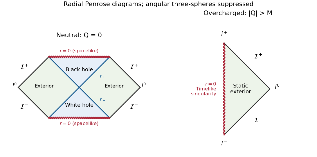
Neutral and overcharged radial Penrose diagrams in five dimensions
. Details. For , the exterior and deep interior are static, while is a trapped or time-reversed band. The outer roots are event horizons for a chosen exterior, and the inner roots are Cauchy horizons. The center is timelike because there. In the exact analytic extension, crossing successive inner and outer horizon branches produces an infinite succession of exterior, trapped, inner-static and white hole blocks. The following finite strip specifies the repetition; it does not terminate the spacetime at the drawing's upper or lower edge.
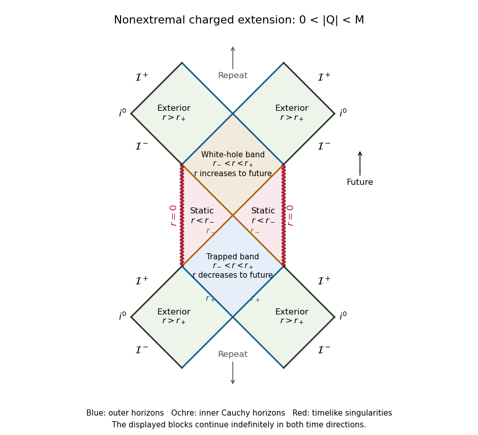
Repeated nonextremal charged blocks with outer and inner horizons and timelike singularities
. Details. For , is nonnegative on both sides of . There is no inter-horizon trapped band. Near the horizon, , so the horizon is an infinite throat end of each static coordinate block. It is null and degenerate, without a regular bifurcation surface. The extension consists of alternating exterior and inner-static blocks, with timelike singularities in the latter. The separate conformal blocks below, together with their future-to-past horizon gluing rule, describe the full repeated extension. The open throat endpoints are ideal boundaries, not additional events where horizon branches meet.
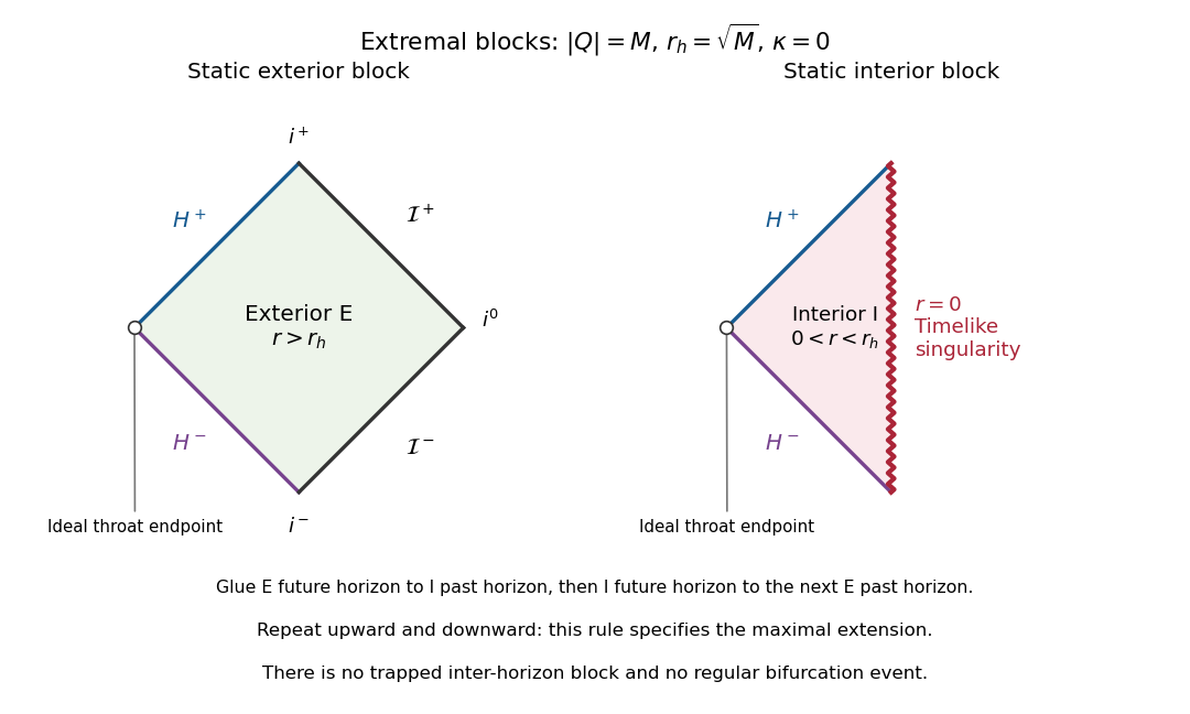
Extremal static conformal blocks and the gluing rule for their maximal extension
. Details. Thus the neutral, strictly subextremal charged, extremal and overcharged cases all have distinct causal structures. These drawings describe the maximal analytic stationary metrics. The additional angular dimension changes areas and curvature falloff, but does not change these radial causal block types.
Past exam of the mathematics course of the University of Cambridge 2004 iii Paper 57 4 ii Solution by Codex 0 Created 2026-10-03 Updated 2026-10-14
Codex 0 Created 2026-10-03 Updated 2026-10-14At a horizon, use in to obtain . A double root therefore requires , and the horizon equation then gives . Conversely at ,Hence . It is a degenerate Killing horizon of an extremal black hole. For distinct charged roots, the normalized signed surface gravities are , so neither is degenerate. The neutral positive-radius horizon is also simple.
Past exam of the mathematics course of the University of Cambridge 2004 iii Paper 57 4 i Solution by Codex 0 Created 2026-10-03 Updated 2026-10-14
Codex 0 Created 2026-10-03 Updated 2026-10-14A positive-radius horizon occurs at a zero of V. Set ; multiplying by gives . Thus real roots require . With , the horizon condition and radii areFor both roots are positive, giving an outer event horizon and an inner Cauchy horizon. For they coincide at . For only is a horizon: the formal root was introduced by multiplication and is the singular origin, where the original expression for V is undefined. For there is no horizon and the central singularity is naked. Each positive root is regular in ingoing coordinates , where the radial metric is .
Past exam of the mathematics course of the University of Cambridge 2004 iii Paper 53 4 4 Solution by Codex 0 Created 2026-10-03 Updated 2026-10-14
Codex 0 Created 2026-10-03 Updated 2026-10-14For known , use nearest-integer stopping for amplitude amplification. SetWriting , the difference between and has absolute value at most . Thus . The Born rule and part 3 giveCount the initial once and the and occurring inside each of the amplification iterates. The number of applications of either preparation unitary is thereforeThe counts separately are applications of and applications of , in addition to applications each of and . This is a quadratic improvement over the mean number of unamplified trials. At an exact rounding tie either nearest iterate meets the probability bound. Knowledge of is used in selecting the stopping time; repeatedly applying without a suitable stopping rule can rotate the state past the good axis and reduce success again. The fact that answers lie in NP supplies verification, but by itself gives no claim that is polynomial in input length.
Past exam of the mathematics course of the University of Cambridge 2004 iii Paper 53 4 3 Solution by Codex 0 Created 2026-10-03 Updated 2026-10-14
Codex 0 Created 2026-10-03 Updated 2026-10-14Choose with . Then and . The matrix found in part 2 is a rotation by in the ordered good-bad plane, with the bad coordinate listed first. The initial coordinate vector is .
After rotations its angle from the bad axis is . Equivalently, multiplication of the displayed matrix and the addition formulas for sine and cosine prove the assertion by induction from . HenceThe Born rule therefore gives good-output probability . This is the geometric mechanism of amplitude amplification: each coherent iteration rotates the already existing good amplitude toward the good axis.
Past exam of the mathematics course of the University of Cambridge 2004 iii Paper 53 4 2 Solution by Codex 0 Created 2026-10-03 Updated 2026-10-14
Codex 0 Created 2026-10-03 Updated 2026-10-14Let project onto the good-output subspace and let , . They are orthonormal because their supporting computational basis strings are disjoint. The verification unitary operator is , so and .
Also . Since , conjugating gives . ThusBoth reflections preserve the span of and : is diagonal there, and the other reflection only adds a multiple of , already in that span. Direct substitution of yieldsThe minus sign in the first image follows from applying before the state reflection. In the ordered basis the matrix isThis exhibits the invariant plane without assumptions about the action of on the other input basis vectors.
Past exam of the mathematics course of the University of Cambridge 2004 iii Paper 53 4 1 Solution by Codex 0 Created 2026-10-03 Updated 2026-10-14
Codex 0 Created 2026-10-03 Updated 2026-10-14For independent attempts, measuring after each application of produces a success with probability . Recognize the answer with the verifier and restart on failure. The number of attempts has a geometric distribution, with . Summing the tail probabilities givesThis counts applications of ; it presumes and a fresh preparation for each attempt. If , neither repetition nor the amplification construction can create a good component from this input.
Pinned article: Introduction to the OurBigBook Project
Welcome to the OurBigBook Project! Our goal is to create the perfect publishing platform for STEM subjects, and get university-level students to write the best free STEM tutorials ever.
Everyone is welcome to create an account and play with the site: ourbigbook.com/go/register. We belive that students themselves can write amazing tutorials, but teachers are welcome too. You can write about anything you want, it doesn't have to be STEM or even educational. Silly test content is very welcome and you won't be penalized in any way. Just keep it legal!
Intro to OurBigBook
. Source. We have two killer features:
- topics: topics group articles by different users with the same title, e.g. here is the topic for the "Fundamental Theorem of Calculus" ourbigbook.com/go/topic/fundamental-theorem-of-calculusArticles of different users are sorted by upvote within each article page. This feature is a bit like:
- a Wikipedia where each user can have their own version of each article
- a Q&A website like Stack Overflow, where multiple people can give their views on a given topic, and the best ones are sorted by upvote. Except you don't need to wait for someone to ask first, and any topic goes, no matter how narrow or broad
This feature makes it possible for readers to find better explanations of any topic created by other writers. And it allows writers to create an explanation in a place that readers might actually find it.
Figure 1. Screenshot of the "Derivative" topic page. View it live at: ourbigbook.com/go/topic/derivativeVideo 2. OurBigBook Web topics demo. Source. - local editing: you can store all your personal knowledge base content locally in a plaintext markup format that can be edited locally and published either:This way you can be sure that even if OurBigBook.com were to go down one day (which we have no plans to do as it is quite cheap to host!), your content will still be perfectly readable as a static site.
- to OurBigBook.com to get awesome multi-user features like topics and likes
- as HTML files to a static website, which you can host yourself for free on many external providers like GitHub Pages, and remain in full control

Figure 2. You can publish local OurBigBook lightweight markup files to either OurBigBook.com or as a static website.
Figure 3. Visual Studio Code extension installation.
Figure 5. . You can also edit articles on the Web editor without installing anything locally. Video 3. Edit locally and publish demo. Source. This shows editing OurBigBook Markup and publishing it using the Visual Studio Code extension. 
- Infinitely deep tables of contents:




All our software is open source and hosted at: github.com/ourbigbook/ourbigbook
Further documentation can be found at: docs.ourbigbook.com
Feel free to reach our to us for any help or suggestions: docs.ourbigbook.com/#contact