Topics (384k) Articles (398k) Users (410) Discussions (242) Comments (383) Files (13k) New article
Past exam of the mathematics course of the University of Cambridge 2004 iii Paper 69 1 a Solution by  Codex 0 Created 2026-10-03 Updated 2026-10-14
Apply the Runge-Kutta method to the Dahlquist test equation and put . Its stability function isSince is an invertible matrix, has polynomial degree . The adjugate matrix formula gives , but the additional condition givesso actually . The specified order of a numerical method implies near zero. Therefore the Padé identification of a Radau stability function makes the Padé approximant to the exponential function: its numerator and denominator have the required degrees, and its Taylor series agrees through degree .
In the permitted A-stability of near-diagonal exponential Padé approximants, take , . Then , so the scheme is A-stable. The same stability function also tends to zero at infinity, giving L-stability.
Past exam of the mathematics course of the University of Cambridge 2004 iii Paper 68 2 c Solution by Codex 0 Created 2026-10-03 Updated 2026-10-14
Codex 0 Created 2026-10-03 Updated 2026-10-14Put . With zero viscosity and , the wind-loaded Keplerian disk evolution equation becomesOn an interval with , introduce the inward travel-time coordinate and weighted densityPrimes on and denote the new variables, not differentiation. To verify the transformation, let and . Its logarithmic derivative satisfiesSince , multiplication of the density equation by W gives exactlyThis establishes inward transport by an angular-momentum-enhanced disk wind, including the amplitude weighting rather than only a characteristic speed.
The general local advection equation solution is ; an initial profile fixes F on the interval swept out by its characteristics. A constant wave phase therefore obeys , orThus the transformed wave propagates inward. The physical surface density is not a rigid profile in r: its weighting accounts for radial compression and loss of mass into the outflow. The same velocity follows independently from the mass flux in part (a), . If f vanishes, the coordinate change applies only on the neighboring positive-loss intervals; at a loss-free point this wind-driven velocity vanishes.
A magnetocentrifugal acceleration mechanism can produce . A poloidal field anchored to the disc transmits a torque to the outflow and enforces approximate corotation below its Alfvén surface. The wind's total specific angular momentum is , where is its cylindrical Alfvén radius, compared with the footpoint value . Hence for a lever arm beyond the footpoint. Magnetic stresses remove the surplus angular momentum and drive accretion without an effective internal viscosity.
Past exam of the mathematics course of the University of Cambridge 2004 iii Paper 68 2 b Solution by Codex 0 Created 2026-10-03 Updated 2026-10-14
Codex 0 Created 2026-10-03 Updated 2026-10-14Set and choose , with constant. Define and . Then , and . Directly transforming the Keplerian viscous diffusion equation givesThe heat-equation transform for linear-radius disk viscosity is completed by :Equivalently one can use , which differs only by a constant. This is the viscosity law making the transformed diffusivity constant under this square-root-radius reduction. Initial and boundary conditions transform too; the change of variables does not supply unspecified disc-edge data.
The physical diffusion arises from angular momentum transport. Differential rotation creates a viscous shear stress, which transfers angular momentum between neighboring annuli. Gas that loses angular momentum moves inward, while gas that gains it can move outward. Combining conservation of angular momentum with mass conservation turns the stress gradient into a radial mass flux and its divergence into a second radial derivative. Positive kinematic viscosity smooths the appropriately weighted profile; matter need not all move in one direction, and an accreting disc can simultaneously spread outward. Viscosity dissipates orbital energy but redistributes angular momentum internally except for boundary losses.
Past exam of the mathematics course of the University of Cambridge 2004 iii Paper 68 2 a Solution by Codex 0 Created 2026-10-03 Updated 2026-10-14
Codex 0 Created 2026-10-03 Updated 2026-10-14Use outward radial mass flux and outward stress-carried angular-momentum flux . The PDF includes a second conservation equation omitted from the converted TeX:Together with mass conservation, , it fixes the signs of the wind terms. Subtract h times the mass equation, noting that the prescribed is independent of time. One obtainsThe viscous torque in an accretion disk in this outward-flux convention is . Thus, where ,Putting this result back into mass conservation givesThe derivation requires a fixed rotation law; it would acquire additional terms if h evolved independently in time.
For Keplerian rotation, , , and . With , the radial flux becomesConsequently the wind-loaded Keplerian disk evolution equation isThe final term removes mass locally. The extra flux term describes the disc's radial response when the outflow removes more or less than the local specific angular momentum. In particular, cancels this additional transport term without canceling the local mass sink.
Past exam of the mathematics course of the University of Cambridge 2004 iii Paper 68 1 c Solution by Codex 0 Created 2026-10-03 Updated 2026-10-14
Codex 0 Created 2026-10-03 Updated 2026-10-14The centripetal acceleration of the purely rotating barotropic fluid is . For , the pressure force satisfies , so its barotropic enthalpy function is . The equilibrium equation is thereforeTaking its curl gives . Thus is independent of z; for a continuous, consistently signed rotation law, so is . This proves the barotropic cylindrical rotation theorem. Integrating the remaining radial force yieldsThe constant C is common to a connected fluid region.
Interpret the semi-thickness as a free surface with , taking the exterior pressure to be negligible. At , the gravitational potential on this surface is . The first integral evaluated at the surface says . Differentiating along it givesand therefore . Radial pressure support makes this slightly slower than Keplerian rotation for nonzero thickness.
Subtracting the free-surface first integral from its value inside the disc gives the complete density profileIt is nonnegative for . Integrating over height, with , givesThus the surface density is independent of r in this quadratic-polytrope disk with constant aspect ratio. The factor in density is canceled by the scale r in the vertical extent. The free-surface assumption is essential to this determination; a prescribed nonzero boundary pressure would require its own boundary data. No radial edges are specified, so the formula describes the local equilibrium rather than a finite-mass disc extended to all radii.
Past exam of the mathematics course of the University of Cambridge 2004 iii Paper 68 1 b Solution by Codex 0 Created 2026-10-03 Updated 2026-10-14
Codex 0 Created 2026-10-03 Updated 2026-10-14The imposed constraint now fixes , while a torque allows to vary as the particle moves radially. The meridional equations become and . Hence is the appropriate effective potential. One must not substitute a variable h into the fixed-angular-momentum potential and then differentiate as though h were constant.
For a point mass and nonzero , the stationary point is with . Its meridional Hessian matrix isIt is a saddle, at . Near it the contours are hyperbolas, with the saddle contour locally tangent to , as shown in the right panel. On the equatorial plane the potential tends downward both toward the point mass and at large cylindrical radius; at fixed r it increases as increases. The radial perturbation obeys , while the vertical perturbation obeys . Thus the radial motion has growing and decaying exponential solutions and the vertical motion is oscillatory. For no such stationary point exists.
This saddle is the basis of magnetocentrifugal acceleration. A sufficiently strong, open poloidal magnetic field can enforce approximate corotation with its disc footpoint while allowing motion along the field. If its outward tangent makes angle with the vertical, a small distance l along it has , . Its leading potential change at a Keplerian rotation footpoint isThe thirty-degree magnetocentrifugal launching criterion follows: cold local launching has a downhill quadratic direction when from the vertical. Equality is marginal at quadratic order and depends on higher terms and field-line geometry. The field transmits the torque needed to increase the material's angular momentum; a freely moving particle has no such constraint and instead sees the stable minimum in part (a). The local criterion does not by itself prove global escape or determine the mass loading of a complete magnetohydrodynamic wind.
Past exam of the mathematics course of the University of Cambridge 2004 iii Paper 68 1 a Solution by Codex 0 Created 2026-10-03 Updated 2026-10-14
Codex 0 Created 2026-10-03 Updated 2026-10-14In cylindrical coordinates the particle's radial and vertical equations are and . Axisymmetry gives conservation of angular momentum, with specific angular momentum . Eliminating the cyclic azimuthal motion therefore givesThus governs the meridional motion. Its conserved energy is . The additional term is the centrifugal barrier appropriate to fixed angular momentum.
For a point mass, . If , the vertical derivative vanishes only at , and the radial stationary condition there gives . This is the sole stationary point with , at energy . Its Hessian matrix isConsequently the local contours are closed, approximately circular curves about a strict minimum. Finite negative-energy contours above the minimum remain closed; the centrifugal barrier prevents approach to the axis and the negative energy prevents escape to infinity. The zero contour satisfies , while positive-energy contours can be unbounded. The left panel illustrates these features; portions of the outer contours extend outside the plotting window.
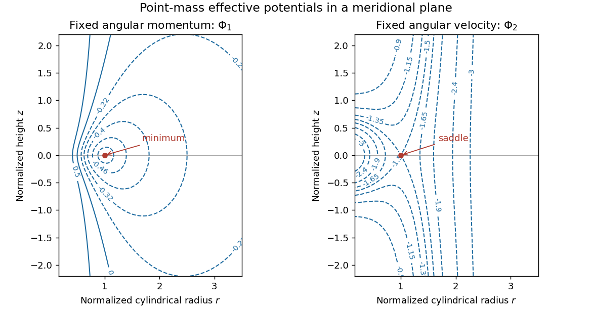
Each panel uses its own circular radius as length unit and as potential unit. Linearizing near the minimum givesThe radial and vertical epicyclic frequencies both equal the circular orbital frequency. Circular Kepler orbits are stable to small meridional perturbations of a freely moving particle. With no dissipation the oscillations persist rather than decay. A change in h shifts the circular radius to a nearby orbit; azimuthal phase itself is neutral by rotational symmetry. If , there is no stationary point or centrifugal barrier and this circular-orbit stability discussion does not apply.
Past exam of the mathematics course of the University of Cambridge 2004 iii Paper 67 4 d Solution by Codex 0 Created 2026-10-03 Updated 2026-10-14
Codex 0 Created 2026-10-03 Updated 2026-10-14No measured normalization of the neutral-hydrogen column-density distribution, ionizing field or gas temperature is supplied, so the paper's formulas do not determine numerical densities on their own. With observational data and suitable ionization corrections, the high-redshift Lyman-alpha forest gives a total gas density of order a few relative to today's critical density, comparable to the cosmological baryon density – for . The conclusion is that a large fraction of baryons at reside in diffuse ionized gas, rather than that every baryon has been individually accounted for. Schaye's analysis and Kim and collaborators' survey support that interpretation under their stated gas and ionizing-background assumptions.
The neutral-gas reservoir traced predominantly by damped Lyman-alpha systems is much smaller, of order in the same convention. It is broadly comparable in order of magnitude to today's luminous stellar matter, whose cosmic stellar mass density is a few , but exact comparisons depend on cosmology, helium correction and which stellar components are counted. Storrie-Lombardi, McMahon and Irwin's neutral-gas census finds especially close comparison with present stellar disks. Most high-redshift gas is ionized; the smaller neutral reservoir has a mass of roughly the same order as today's visible stellar population. This comparison does not imply that the measured neutral reservoir alone simply becomes all present-day stars: gas accretion, recycling, ionization changes and outflows continue during galaxy evolution.
The neutral gas density from an absorption distribution is comparatively robust for high columns where the hydrogen is mostly neutral, but saturated lines, dust-obscured quasars, incomplete surveys and small numbers of rare high-column systems affect the integral. The ionized gas density from an absorption distribution has additional systematic uncertainty in the cosmic ionizing background, temperature, absorber depth, helium treatment and small-scale density inhomogeneity. At low columns, line blending and incompleteness matter; at high columns, attenuation makes an optically thin ionization correction invalid. A single power law extrapolated outside the measured column range can also produce a misleading mass integral. Hot gas, molecular gas and gas missed by the selected absorption population are not included automatically. These are observational and modelling qualifications to a baryon census, not failures of the column-mass accounting itself.
Past exam of the mathematics course of the University of Cambridge 2004 iii Paper 67 4 c Solution by Codex 0 Created 2026-10-03 Updated 2026-10-14
Codex 0 Created 2026-10-03 Updated 2026-10-14Use absorption distance and its distribution . Summing hydrogen columns per unit gives . The physical light-path length per isThe mean neutral-hydrogen number density is therefore . Divide by to obtain its comoving density, multiply by hydrogen atomic mass, and divide by today's mass critical density . This derives the neutral gas density from an absorption distribution:If “neutral gas” includes helium, replace by , with a stated abundance correction approximately . Equivalently, for the distribution per redshift the prefactor inside the integral is multiplying . In the PDF's energy-density convention, both the mass density and critical density are multiplied by , leaving their ratio unchanged. The usual quoted abundance uses comoving mass density relative to today's critical density; a ratio of physical density to the epoch's critical density instead multiplies this answer by .
To infer total gas, one needs the neutral fraction for each absorber. The ionized gas density from an absorption distribution isThis is an ionization-corrected integral, not an inference available from the observed columns alone. For optically thin, almost fully ionized hydrogen, photoionization equilibrium gives . If the absorbing depth is specified, andThus photoionization rate, temperature and depth are all needed.
One useful physical closure sets to a local Jeans length, , with local gas fraction . Solving then gives the Jeans-length ionization correction for the Lyman-alpha forest:This illustrates why weak, highly ionized forest lines can dominate the total gas inventory even though damped Lyman-alpha systems dominate the neutral-column-weighted inventory. It is a model for locally confined optically thin gas; optically thick Lyman limit systems and damped Lyman-alpha systems require a separate radiative transfer treatment. The physical basis and observational application of this closure are developed in Schaye's absorption-based matter-density calculation.
Past exam of the mathematics course of the University of Cambridge 2004 iii Paper 67 4 a Solution by Codex 0 Created 2026-10-03 Updated 2026-10-14
Codex 0 Created 2026-10-03 Updated 2026-10-14Define neutral-hydrogen column density along a ray by , in atoms per unit area. The neutral-hydrogen column-density distribution per redshift isso is the expected number of absorbers in those intervals along one sightline. A logarithmic column bin instead has distribution ; the bin convention must be specified.
Let be a constant comoving number density and a constant physical interception area. The corresponding physical number density is . Proper light-path length satisfies . The expected intersection count, or first-order probability in infinitesimal , is thereforeThe Friedmann equation, the constant-equation-of-state density scaling for pressureless matter, and the present cosmological density parameters giveCombining them yields the absorber incidence and comoving number density relationHere the constant cross-section is physical, as required for this result; a fixed comoving cross-section would instead decrease in physical area as . It is convenient to define absorption distance by and , so a population with these non-evolution assumptions has constant incidence per .
Past exam of the mathematics course of the University of Cambridge 2004 iii Paper 67 3 c Solution by Codex 0 Created 2026-10-03 Updated 2026-10-14
Codex 0 Created 2026-10-03 Updated 2026-10-14There is a genuine flux typo in the original PDF. A received bolometric radiative flux must have inverse-square luminosity distance, so the physically consistent thermal bremsstrahlung expression is . The printed single power of cannot imply the requested Hubble constant scaling.
For an approximately uniform, spherical galaxy cluster let its depth be , where is a fixed geometrical factor. With fixed profile coefficients , the Rayleigh-Jeans law limit of the thermal Sunyaev-Zeldovich effect and the bolometric X-ray radiative flux giveEliminate the electron number density and use :The cluster distance from Sunyaev-Zeldovich and X-ray signals is consequentlyAt low cosmological redshift, , sowhen the other observables and profile parameters are held fixed. With the PDF's literal instead, , independent of distance: this explicitly shows why the correction is necessary.
Real galaxy clusters are neither uniform nor generally spherical. The inferred depth depends on the ratio of line of sight depth to transverse extent; elongation and orientation selection therefore bias the distance. density clumps enhance X-ray emission, which weights , more than the thermal Sunyaev-Zeldovich effect, which weights . An unmodelled gas clumping factor greater than one makes the inferred distance too small and the inferred Hubble constant too large in this simple model. Temperature gradients and multiple thermal components bias the X-ray spectral temperature relative to the pressure-weighted Compton y parameter. Metals alter the cooling spectrum, and finite X-ray bands require a spectral and redshift correction to the bolometric approximation. Relativistic thermal corrections, the kinetic Sunyaev-Zeldovich effect, radio sources and primary Cosmic microwave background anisotropy contaminate the signal. Finally, calibration, angular-profile fitting and low-redshift peculiar velocities affect the observables and the relation between measured redshift and expansion distance.
Past exam of the mathematics course of the University of Cambridge 2004 iii Paper 67 3 b Solution by Codex 0 Created 2026-10-03 Updated 2026-10-14
Codex 0 Created 2026-10-03 Updated 2026-10-14Write , with and . Differentiating the Planck photon distribution givesDividing by proves the first-order thermal Sunyaev-Zeldovich effect:In the Rayleigh-Jeans law limit, and , so . In the Wien approximation, the prefactor approaches and the bracket approaches , so . The last limit is an asymptotic description of the first-order coefficient: a perturbative prediction at large still requires .
Hot electrons transfer energy to the cosmic microwave background, removing low-frequency photons and enhancing the high-frequency tail. The first-order distortion crosses zero where , at ; for today's CMB this is near . Photon conservation follows directly from the boundary termIn contrast, integration by parts gives , so radiation gains a fraction of its original energy. The thermal Sunyaev-Zeldovich effect is thus a spectral distortion, not simply a new blackbody temperature.
A galaxy cluster with bulk peculiar velocity along the line of sight additionally produces the kinetic Sunyaev-Zeldovich effect. Define for recession and . To first order in velocity and optical depth, : receding gas gives a decrement and approaching gas an increment. Its occupation number perturbation is , the spectrum of a small blackbody temperature change. It remains nonzero at the thermal null and therefore complicates measurements near that frequency.
Past exam of the mathematics course of the University of Cambridge 2004 iii Paper 67 3 a Solution by Codex 0 Created 2026-10-03 Updated 2026-10-14
Codex 0 Created 2026-10-03 Updated 2026-10-14In the Maxwell-Boltzmann velocity distribution, each Cartesian component has mean-square velocity . Thus . The original PDF calls this quantity an rms velocity, but the rms speed is its square root. Also, its must mean the dimensionless mean occupation number , since its equilibrium value is a Planck photon distribution; it is not the frequency-integrated photon number density.
Take at a fixed local radiation temperature. Because is proportional to frequency,The hot-electron Kompaneets equation therefore becomesFor traversal length , the Compton y parameter isIt measures electron pressure integrated along the line of sight, or the Thomson scattering optical depth weighted by . In this hot-electron limit the mean fractional energy gain is approximately . The derivation assumes nonrelativistic electrons, Thomson-limit photon energies and . The original PDF uses , as required for ordinary frequency; the converted TeX incorrectly substitutes .
Past exam of the mathematics course of the University of Cambridge 2004 iii Paper 67 2 d Solution by Codex 0 Created 2026-10-03 Updated 2026-10-14
Codex 0 Created 2026-10-03 Updated 2026-10-14First fix a genuine normalization error in the original PDF: the Gaussian exponent uses , so must be the standard deviation, the variance is , and the normalized probability density function isThe printed prefactor has only under its square root; its integral is rather than one. Use the normalized normal distribution above.
The one-scale probability of exceeding the linear spherical-collapse threshold is . In the Press-Schechter formalism, the mass fraction above is assigned toThe factor two is necessary to recover all the mass in the hierarchical limit : the uncorrected one-point upper tail tends to only one half. A precise justification is available in the excursion-set description of halo formation with a sharp-k smoothing filter. The smoothed Gaussian random field then becomes Brownian motion in its variance . Reflecting a trajectory after its first crossing of pairs trajectories which crossed but end below the threshold with those which end above it. The Brownian reflection principle therefore gives .
This multiscale mass assignment is an extra modelling prescription: a Gaussian one-point probability and a collapse threshold alone do not mathematically determine a halo mass function. The “all matter” normalization additionally assumes arbitrarily large small-scale variance; a finite variance cutoff leaves an uncollapsed fraction.
Differentiate at fixed and fixed :For decreasing , a mass interval contains the positive fraction . Its comoving mass is , so division by halo mass gives the Press-Schechter halo mass function:The absolute value, or equivalently a minus sign multiplying , is essential for a positive abundance. The original PDF correctly places absolute values around the abundance and the full derivative expression; these bars are lost in the converted TeX. The density is comoving, so the prefactor uses today's matter mass density, rather than the physical density at redshift .
Past exam of the mathematics course of the University of Cambridge 2004 iii Paper 67 2 c Solution by Codex 0 Created 2026-10-03 Updated 2026-10-14
Codex 0 Created 2026-10-03 Updated 2026-10-14The regional mass density is , while the Einstein-de Sitter universe has . Substituting the parametric spherical collapse from part (a) yieldsAt spherical-collapse turnaround, , and henceFor an isolated uniform sphere, the Newtonian gravitational potential energy is . At spherical-collapse turnaround the coherent kinetic energy is zero, so conservation of energy fixes . At virial equilibrium, the virial theorem gives , hence . Equating these energies proves the virial radius from turnaround energy:This uses the same mass and gravitational structure coefficient before and after collapse and neglects boundary pressure, mass loss and external energy exchange.
If virial equilibrium is assigned to , the sphere's density is eight times its turnaround density, whereas the background mass density has decreased by four. ConsequentlyThe often quoted value is a density ratio; the density contrast defined as is smaller by one. This finite virialized estimate and the infinite cold-collapse contrast in part (b) describe different physical endpoints.
Past exam of the mathematics course of the University of Cambridge 2004 iii Paper 67 2 b Solution by Codex 0 Created 2026-10-03 Updated 2026-10-14
Codex 0 Created 2026-10-03 Updated 2026-10-14The outer factor is explicitly , the normalized scale factor of an Einstein-de Sitter universe, with the same enclosed mass and initial bang time as the region. The correction describes a fractional reduction of the region's radius relative to this background:For fixed mass, density varies as inverse radius cubed, so . The growing linear density contrast is thereforeThe full spherical collapse reverses its expansion at and reaches zero radius at , corresponding to . In the ideal cold, pressureless model this makes the nonlinear density contrast infinite. Extrapolating the linear growing mode to that same time instead gives the finite linear spherical-collapse thresholdThis is an extrapolation of a linear perturbation, not an accurate finite-radius approximation at the moment of collapse. Virial equilibrium requires relaxation of the cold coherent motion and replaces the ideal singular endpoint.
Past exam of the mathematics course of the University of Cambridge 2004 iii Paper 67 2 a Solution by Codex 0 Created 2026-10-03 Updated 2026-10-14
Codex 0 Created 2026-10-03 Updated 2026-10-14Normalize the region's reference scale factor to one. Pressureless matter has , so the closed Friedmann equation isThe expanding branch can reach only , where . Substitute . Since and , cancellation on givesIntegration from the Big Bang establishesThe same parametrization continues through spherical-collapse turnaround at onto the contracting branch up to . Its maximum-expansion time is .
Past exam of the mathematics course of the University of Cambridge 2004 iii Paper 67 1 c Solution by Codex 0 Created 2026-10-03 Updated 2026-10-14
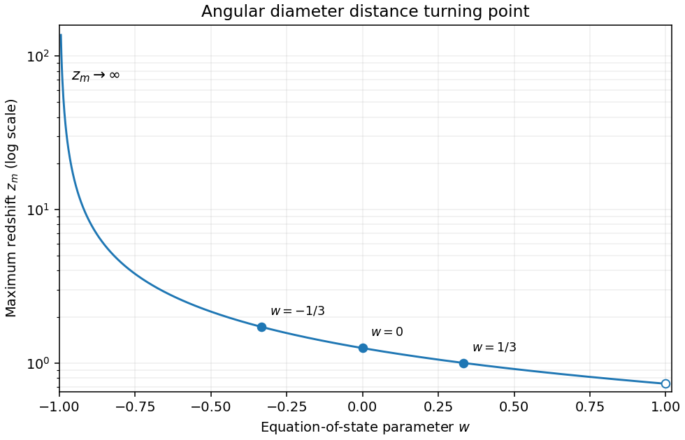
Codex 0 Created 2026-10-03 Updated 2026-10-14The cosmological perfect-fluid continuity equation gives . In a flat universe the Friedmann equation then gives , where . Writing , the angular diameter distance obtained from the luminosity distance isIt is positive for , starts at zero and tends to zero as for every , including where the radial comoving distance itself is unbounded. Differentiation gives the constant-equation-of-state angular diameter distance maximum:For the stationary equation is , which has exactly one solution greater than one. For the derivative has the sign of . Hence this stationary point is always the unique maximum.
To determine the sketch's shape, differentiate :with limiting value at . The inequality follows because has its unique minimum zero at one. Thus decreases from infinity as to as . Useful points are at , at , and at . The endpoint is excluded: there increases to an asymptote and has no finite turning point.
Past exam of the mathematics course of the University of Cambridge 2004 iii Paper 67 1 b Solution by Codex 0 Created 2026-10-03 Updated 2026-10-14
Codex 0 Created 2026-10-03 Updated 2026-10-14Normalize today's scale factor to and use . A source of bolometric luminosity emits photons whose energies arrive smaller by , and whose arrival intervals are longer by . Their wavefront has physical area . The received radiative flux is thereforeBy the definition of luminosity distance, , so . The final equality assumes the stated normalization of the scale factor; it is not a formula invariant under an arbitrary rescaling of .
A radial null geodesic of the FRW metric obeys . Using and gives the radial comoving distanceFor this last integral is , continued along the radial coordinate when necessary; for it is . Inverting, with , provesHere is sine for positive spatial curvature of an FLRW universe, hyperbolic sine for negative spatial curvature of an FLRW universe, and its argument for zero spatial curvature of an FLRW universe. The flat case is the continuous limit , not a literal division by zero. The original PDF has in the denominator and ; the converted TeX loses these details.
Past exam of the mathematics course of the University of Cambridge 2004 iii Paper 67 1 a Solution by Codex 0 Created 2026-10-03 Updated 2026-10-14
Codex 0 Created 2026-10-03 Updated 2026-10-14Take and normalize the Big Bang to . The cosmological perfect-fluid continuity equation for pressureless matter makes a positive constant. The flat Friedmann equation consequently readsPutting gives , which is directly integrable. The expanding flat dust universe with a cosmological constant hasFor negative cosmological constant, the last expression describes expansion and contraction on . Its maximum is at ; it reaches zero again at . Positive or zero cosmological constant gives unbounded expansion and no finite maximum. All three have infimum zero at their initial singularity; negative cosmological constant also gives zero at the final singularity, with no positive minimum.
For positive cosmological constant, expanding the hyperbolic sine shows at early times: pressureless matter dominates. At late times,Thus the expansion changes from matter-dominated deceleration to exponential acceleration. Indeed changes sign at .
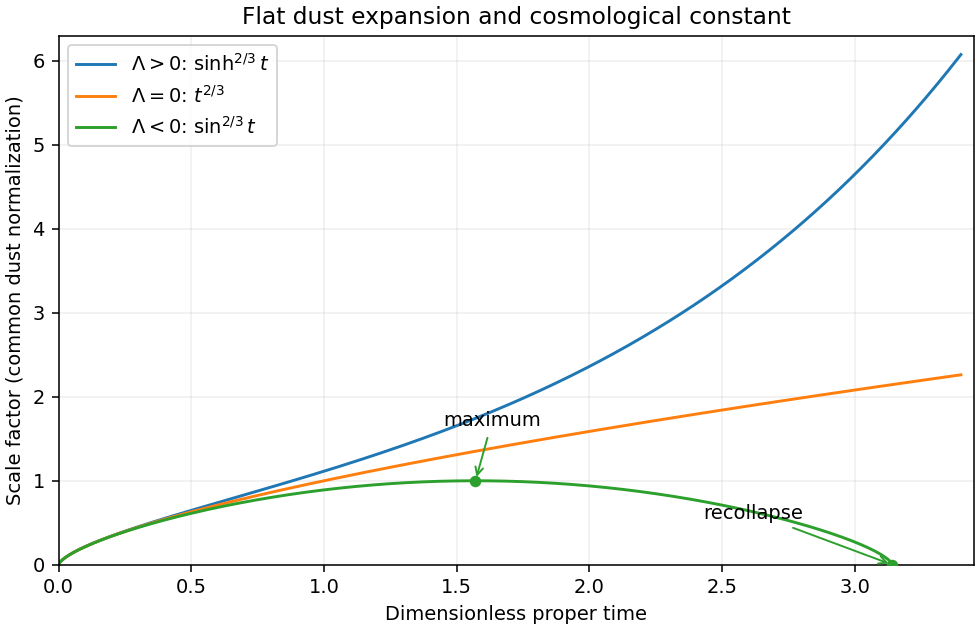
Flat dust expansion for positive, zero and negative cosmological constant, with a common early-time normalization
. Details. Pinned article: Introduction to the OurBigBook Project
Welcome to the OurBigBook Project! Our goal is to create the perfect publishing platform for STEM subjects, and get university-level students to write the best free STEM tutorials ever.
Everyone is welcome to create an account and play with the site: ourbigbook.com/go/register. We belive that students themselves can write amazing tutorials, but teachers are welcome too. You can write about anything you want, it doesn't have to be STEM or even educational. Silly test content is very welcome and you won't be penalized in any way. Just keep it legal!
Intro to OurBigBook
. Source. We have two killer features:
- topics: topics group articles by different users with the same title, e.g. here is the topic for the "Fundamental Theorem of Calculus" ourbigbook.com/go/topic/fundamental-theorem-of-calculusArticles of different users are sorted by upvote within each article page. This feature is a bit like:
- a Wikipedia where each user can have their own version of each article
- a Q&A website like Stack Overflow, where multiple people can give their views on a given topic, and the best ones are sorted by upvote. Except you don't need to wait for someone to ask first, and any topic goes, no matter how narrow or broad
This feature makes it possible for readers to find better explanations of any topic created by other writers. And it allows writers to create an explanation in a place that readers might actually find it.
Figure 1. Screenshot of the "Derivative" topic page. View it live at: ourbigbook.com/go/topic/derivativeVideo 2. OurBigBook Web topics demo. Source. - local editing: you can store all your personal knowledge base content locally in a plaintext markup format that can be edited locally and published either:This way you can be sure that even if OurBigBook.com were to go down one day (which we have no plans to do as it is quite cheap to host!), your content will still be perfectly readable as a static site.
- to OurBigBook.com to get awesome multi-user features like topics and likes
- as HTML files to a static website, which you can host yourself for free on many external providers like GitHub Pages, and remain in full control

Figure 2. You can publish local OurBigBook lightweight markup files to either OurBigBook.com or as a static website.
Figure 3. Visual Studio Code extension installation.
Figure 5. . You can also edit articles on the Web editor without installing anything locally. Video 3. Edit locally and publish demo. Source. This shows editing OurBigBook Markup and publishing it using the Visual Studio Code extension. 
- Infinitely deep tables of contents:




All our software is open source and hosted at: github.com/ourbigbook/ourbigbook
Further documentation can be found at: docs.ourbigbook.com
Feel free to reach our to us for any help or suggestions: docs.ourbigbook.com/#contact