Topics (384k) Articles (398k) Users (410) Discussions (242) Comments (383) Files (13k) New article
Past exam of the mathematics course of the University of Cambridge 2004 iii Paper 61 2 a Solution by  Codex 0 Created 2026-10-03 Updated 2026-10-14
Write . In terms of Wirtinger derivatives, the elliptic equation is . If , its coefficients are and . Direct differentiation givesTherefore , proving that is a closed differential one-form. The parameter restriction makes its coefficients well defined.
Past exam of the mathematics course of the University of Cambridge 2004 iii Paper 61 1 f Solution by Codex 0 Created 2026-10-03 Updated 2026-10-14
Codex 0 Created 2026-10-03 Updated 2026-10-14The algebraic change of variables still works for , but the transformed initial data are now multiplied by . Mere decay of does not ensure existence of the Half-range Fourier transform used above. For example, with gives a growing transformed profile.
There is also a genuine stability distinction. On the whole line a real-frequency mode of the original equation evolves with factorIts modulus is , so positive amplifies arbitrarily high frequencies rather than damping them. Thus the formal gauge equivalence does not justify the same unweighted Sobolev well-posedness conclusion. Weighted or more strongly decaying data and corresponding contour changes may allow particular solutions; the assumptions stated for the negative- construction cannot simply be reused.
Past exam of the mathematics course of the University of Cambridge 2004 iii Paper 61 1 e Solution by Codex 0 Created 2026-10-03 Updated 2026-10-14
Codex 0 Created 2026-10-03 Updated 2026-10-14First remove the observation time from the spectral amplitude. For any fixed horizon , replace by in the formula of part (d). The difference in the boundary integral is proportional toFor every , this integrand is holomorphic inside , where , and decays on its large closing arcs. The Cauchy integral theorem makes the difference zero. This finite-horizon extension of a boundary transform therefore gives the time-independent spectraAll observation-time dependence is now in .
When the boundary history is sufficiently decaying, the natural long-time version isThe integral converges in for bounded boundary data and on its boundary for integrable histories; otherwise one must state an Abel prescription or a suitable temporal growth assumption. Arbitrary smooth need not have such an infinite-time transform. The finite-horizon formula remains exact without that extra assumption, and the source alone does not prescribe a universal long-time limit.
A useful further decomposition, if with integrable , isThis separates the persistent forcing from the transient spectrum. The pole at , where , accounts for the decaying stationary profile ; that profile also follows directly from , spatial decay and its boundary value. For the remaining oscillatory integrals the phase is . At a fixed ray , its stationary points satisfy , or . These time-independent amplitudes expose precisely the poles and saddle points used in the method of steepest descent; allowable deformations must also respect the analyticity strip of the initial transform.
Past exam of the mathematics course of the University of Cambridge 2004 iii Paper 61 1 d Solution by Codex 0 Created 2026-10-03 Updated 2026-10-14
Codex 0 Created 2026-10-03 Updated 2026-10-14The cubic dispersion symmetry with negative transport supplies two other roots of :Both lie in the lower half-plane when . For example this is immediate at large positive imaginary . A root could leave that half-plane only by becoming real, where , contradicting . Connectedness of completes the argument; a coalescence merely exchanges the two roots.
Evaluate the global relation at these roots. Because their dispersion values equal , the same boundary transforms occur, andInterpolate this linear polynomial in at . Defineand similarly . Substitution givesIndeed, interpolation of yields , which proves the coefficient after subtracting .
The final-state term has zero contour integral. After cancelling its integrand is , holomorphic in and decaying upon closing the contour upward for . The possible square-root singularities are removable: the expression is unchanged by exchanging the roots, and when they coalesce at , its limit is , with the same formula for the final-state transform. Thus the Cauchy integral theorem eliminates this unknown term.
We obtain the fully specified Dirichlet spectral formula for Airy flow with negative transportOnly the initial Fourier transform and the given boundary-value time transform remain.
Past exam of the mathematics course of the University of Cambridge 2004 iii Paper 61 1 c Solution by Codex 0 Created 2026-10-03 Updated 2026-10-14
Codex 0 Created 2026-10-03 Updated 2026-10-14Use the negative-exponential Half-range Fourier transformFor the boundary traces , define finite-time spectral boundary transforms . Integrating the conservation law in and then time gives the global relationThe plus sign of the boundary contribution follows because the integrated flux is .
Fourier inversion consequently gives a real-line initial integral plus a boundary integral. To put the latter in the complex plane, defineOrient from the left upper infinity, through , to the right upper infinity, with on the left. Each is entire, and in the region between the real axis and this contour, . The causal factors are bounded there and decays for . The Cauchy integral theorem, with the usual large-arc limiting argument, deforms the boundary integral to giveInitial smoothness, spatial decay and corner compatibility justify inversion; if necessary the integrals are first regularized before contour deformation. The unknown Neumann-type traces will be removed by the global relation.
Past exam of the mathematics course of the University of Cambridge 2004 iii Paper 61 1 b Solution by Codex 0 Created 2026-10-03 Updated 2026-10-14
Codex 0 Created 2026-10-03 Updated 2026-10-14Put and define the spectral fluxWriting , division of the proposed divergence form by gives . Direct differentiation yieldsThe last term cancels , so the divergence form is exactly the normalized partial differential equation. This calculation fixes both the sign of the dispersion relation and the sign of the boundary flux used below.
Past exam of the mathematics course of the University of Cambridge 2004 iii Paper 61 1 a Solution by Codex 0 Created 2026-10-03 Updated 2026-10-14
Codex 0 Created 2026-10-03 Updated 2026-10-14Set , , and use the gauge reduction of a third-order half-line equationThe spatial differential operator acting on is obtained by replacing with . Its second-derivative coefficient vanishes. The first-derivative coefficient is , and the constant coefficient is . The time derivative supplies , so all constant terms cancel and the remaining equation is .
The transformed initial condition and Dirichlet boundary data are thereforeCompatibility at the corner is preserved. Since , this exponential gauge improves the spatial decay of the initial data, which supports convergence of its Half-range Fourier transform.
Past exam of the mathematics course of the University of Cambridge 2004 iii Paper 60 4 d Solution by Codex 0 Created 2026-10-03 Updated 2026-10-14
Codex 0 Created 2026-10-03 Updated 2026-10-14For , the graph of has a positive maximum at and a negative minimum at . The central branch is stable, while the formal outer branches are unstable. Near the gluing point only the stable central branch is relevant: it crosses from negative to positive , representing the stable two-to-one gluing described in part (b). The formal full power-law diagram has three fixed points between its two large saddle-node bifurcations.
For , the positive branch has its minimum at , while the negative branch has its maximum at . The inner pieces are unstable and outer pieces stable. In the gluing-map cusp interval there is a stable negative branch, a stable positive branch, and an unstable central branch; the unstable branch passes through the singular gluing point with opposite sign to . Outside the gluing-map cusp just one stable outer branch remains. The lower panels of the figure plot these diagrams in fold-scaled variables; dashed lines denote instability and solid lines dynamical stability. Neither diagram has a flip bifurcation, since the scalar derivative is positive wherever defined.
Past exam of the mathematics course of the University of Cambridge 2004 iii Paper 60 4 c Solution by Codex 0 Created 2026-10-03 Updated 2026-10-14
Codex 0 Created 2026-10-03 Updated 2026-10-14For a fixed point write . A saddle-node bifurcation requires both and . For these conditions giveThe second derivative is nonzero at either nonzero saddle-node bifurcation, making it an ordinary saddle-node bifurcation. For , defineThe saddle-node bifurcations occur at and , and three scalar fixed points coexist for . The two outer branches have fixed-point multiplier below one and are stable, while the middle branch is unstable. Negative points lift to two symmetry-related limit cycles, so these scalar branch counts need not equal the number of flow limit cycles. The cusp records coexistence of distinct return-map branches; even outside it a negative branch represents a symmetry-related pair of flow cycles.
If , , thenThis exponentially narrow region ends in a gluing-map cusp at . At its boundaries the graph of is tangent to the diagonal at or , as shown below. At exactly , and gives one stable fixed point for nonzero .
For , the formal saddle-node bifurcation radius is , and the corresponding saddle-node bifurcation parameters also diverge. Thus the near-origin gluing-map cusp lies on the side; the formal large saddle-node bifurcations of the power-law formula on the other side are outside the local gluing-map approximation. They must not be drawn as a second small gluing-map cusp near the origin.
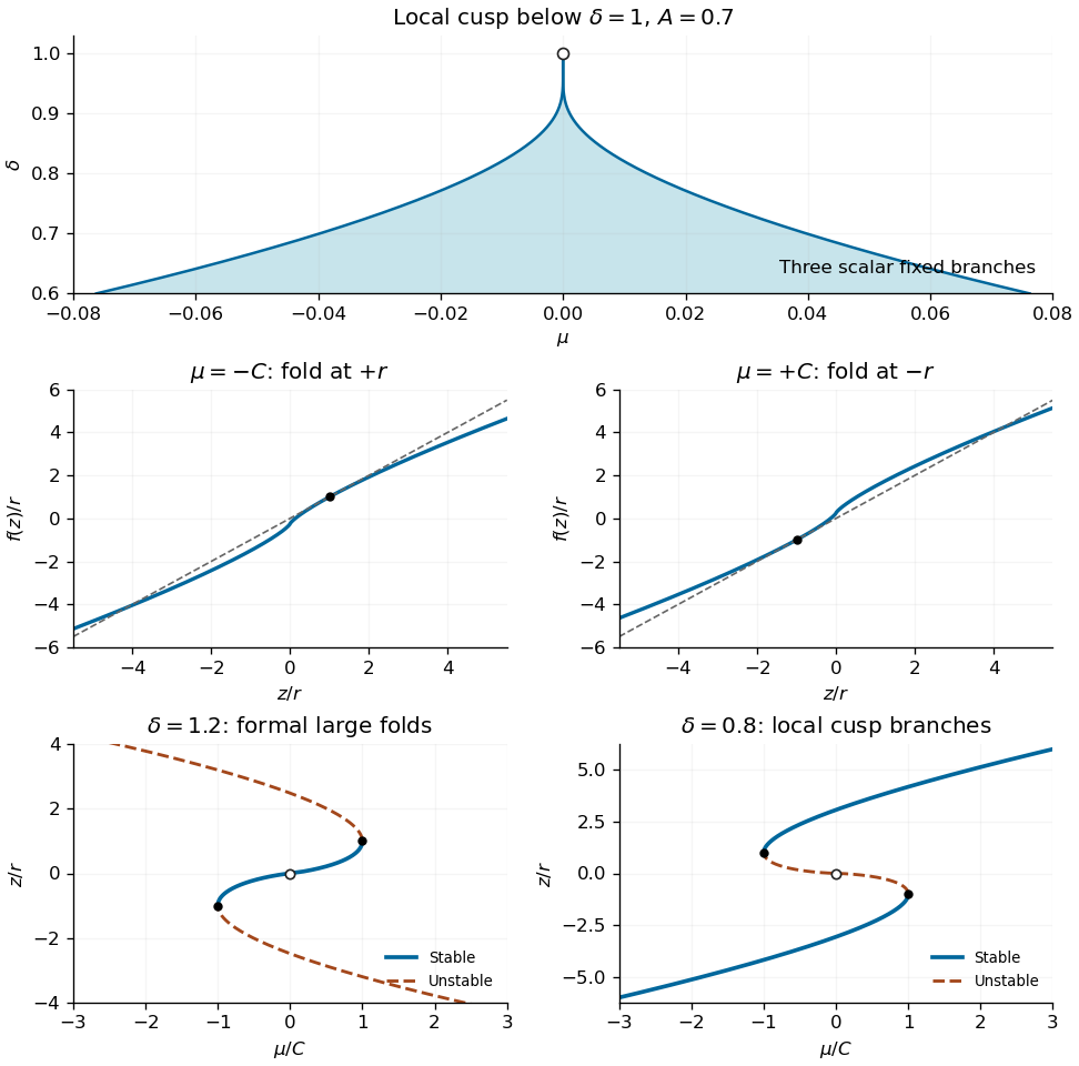
Exponentially narrow gluing-map cusp, tangencies at its two fold boundaries, and stable and unstable fixed-point diagrams on either side of delta one
. Details. Past exam of the mathematics course of the University of Cambridge 2004 iii Paper 60 4 b Solution by Codex 0 Created 2026-10-03 Updated 2026-10-14
Codex 0 Created 2026-10-03 Updated 2026-10-14Let a scalar fixed point have magnitude . If , then and have the same sign; the two lifts are the fixed points and . If , their signs are opposite, and the lift is the period-two orbit . The scalar fixed-point multiplier isThe two-return fixed-point multiplier of the period-two lift is , so in either case dynamical stability requires . The negative fixed point represents one of two mirror-related single-lobe periodic orbits in the flow, whereas the positive fixed point represents a double-lobe periodic orbit.
For , the nearby fixed point is and its fixed-point multiplier tends to zero. Thus two stable single-lobe limit cycles for glue into one stable double-lobe limit cycle for . Their periods diverge as the separatrix is approached; is not a finite-period limit cycle.
For , the small branch instead satisfies and its fixed-point multiplier tends to infinity. Hence one unstable double-lobe limit cycle on splits into two unstable single-lobe limit cycles on . Additional finite-size stable branches depend on the surrounding map; near the resonance with they are resolved by the saddle-node bifurcations in part (c).
Past exam of the mathematics course of the University of Cambridge 2004 iii Paper 60 4 a Solution by Codex 0 Created 2026-10-03 Updated 2026-10-14
Codex 0 Created 2026-10-03 Updated 2026-10-14After one iteration , so work on that invariant sign sheet. For ,since and . This is the signed gluing-map reduction. If an arbitrary initial value of is admitted, the formula applies after that first iterate, not before it. The point represents a separatrix at which the original flow return is singular, even though the scalar map can be extended continuously there.
Past exam of the mathematics course of the University of Cambridge 2004 iii Paper 60 3 c Solution by Codex 0 Created 2026-10-03 Updated 2026-10-14
Codex 0 Created 2026-10-03 Updated 2026-10-14The primary vorticity Jacobian determinant vanishes because . The quadratic temperature Jacobian determinant isThe mean temperature correction therefore obeys . Its Jacobian determinant with the primary streamfunction isProjecting on the retained primary modes gives, with ,For a nonzero steady roll, and . Substitution in the second equation gives, within this truncation,The positive denominator ensures branches only on the supercritical side for every . To verify dynamical stability as well as existence, the critical right eigenvector is ; normalizing the left eigenvector gives linear eigenvalue derivativeQuadratic slaving gives , and projection of its feedback gives the cubic amplitude equationIts nonzero branches are stable in the center direction, while all other eigenvalues remain negative at a simple onset. Reflection about the mid-width sends , so the bifurcation is a supercritical pitchfork bifurcation for all , in the generic case of a single critical roll mode.
The cubic saturation of quasistatic magnetoconvection result is identical in Fourier truncation and perturbation theory at the orders needed here. At quadratic order the only forced mode is precisely the retained horizontally uniform temperature mode. At cubic order its feedback projects on the primary mode with the same coefficient. The generated third vertical harmonic is orthogonal to that primary projection and contributes only to higher-order corrections. Thus both methods give the same linear threshold and cubic solvability condition; the truncated finite-amplitude branch is not an exact solution of the full PDE at all amplitudes.
Past exam of the mathematics course of the University of Cambridge 2004 iii Paper 60 3 b Solution by Codex 0 Created 2026-10-03 Updated 2026-10-14
Codex 0 Created 2026-10-03 Updated 2026-10-14Put and . ThenThe minimizing condition isIts left side increases strictly for and the neutral curve diverges at both ends, so there is a unique global minimum. For large , and the leading balance is . ThereforeThis is the strong-field wavenumber selection in magnetoconvection scaling. In a box of fixed width one compares the two admissible horizontal wavenumbers bracketing the continuum optimum.
Past exam of the mathematics course of the University of Cambridge 2004 iii Paper 60 3 a Solution by Codex 0 Created 2026-10-03 Updated 2026-10-14
Codex 0 Created 2026-10-03 Updated 2026-10-14Write and use modes satisfying all boundary conditions,The quadratic temperature distortion is retained for the saturation calculation; it does not enter the linear onset. Substitution of the primary modes givesThe determinant vanishes whenThe trace is . Thus no conjugate eigenvalues can cross the imaginary axis away from zero, and the initial instability is stationary, not oscillatory. Indeed for the discriminant is . This is quasistatic vertical-field magnetoconvection: there is no independent magnetic evolution mode that could produce a magnetic-thermal Hopf bifurcation instability.
For a fixed box the other allowed horizontal wavenumbers are , and the actual first threshold is the minimum of their corresponding values. Vertical index replaces by and strictly increases the threshold at fixed horizontal wavenumber, so is selected. The displayed formula describes the prescribed fundamental roll; part (b) optimizes its width.
Past exam of the mathematics course of the University of Cambridge 2004 iii Paper 60 2 b Solution by Codex 0 Created 2026-10-03 Updated 2026-10-14
Codex 0 Created 2026-10-03 Updated 2026-10-14Put . The planar vector field and its equilibrium eigenvalue data areFor a nonzero equilibrium, use to rewrite the determinant as . These formulas determine the local bifurcations of the imperfect soft Duffing-van der Pol oscillator directly.
When , the origin is a saddle equilibrium for and has determinant for ; the two equilibria are saddle equilibria. They meet the origin in a symmetry-protected pitchfork bifurcation at for . At the origin undergoes a supercritical Hopf bifurcation. To determine criticality, take : averaging gives , so the stable small limit cycle has .
The potential energy of the conservative part and the exact energy balance areAt zero imperfection the stable limit cycle grows to a heteroclinic cycle connecting the two outer saddle equilibria. Near the double-zero point its leading connection curve can be calculated, rather than inferred just from symmetry. In the Hamiltonian system limit the heteroclinic orbit is , andThe weak-damping persistence condition is therefore , not an exact formula at order-one parameters.
Now take ; negative imperfection reflects the phase portrait. The pitchfork bifurcation unfolds into a transcritical bifurcation crossing at and a saddle-node bifurcation at . The latter occurs at . Between those values the origin and are saddle equilibria, while lies in and is a sink or source according to the trace. At , exchanges its saddle equilibrium/non-saddle character with the origin. The double-zero points are now at and .
The original Hopf bifurcation line remains, still supercritical. A second Hopf bifurcation curve occurs on the intermediate nonzero equilibrium:It is important not to assign the same criticality to its entire length. Write , so . Around that center the restoring quadratic coefficient is , the damping linear coefficient is , and . The Hopf criticality for an asymmetric Lienard center calculation gives cubic amplitude coefficientHence it is supercritical for and subcritical for , with a generalized Hopf bifurcation point at . Higher-order terms are needed exactly there. For small imperfection the leading quintic coefficient is positive: writing and using the coordinate that normalizes the potential energy, , with and , the coefficient of in at vanishing cubic coefficient is . Weak-damping averaging therefore supplies the nearby saddle-node bifurcation of stable and unstable limit cycles in the generalized Hopf bifurcation unfolding. None of these small features intersects either requested parameter line.
Globally, the two saddle equilibrium barriers are no longer equal. Their leading energy difference is . The two one-way connections consequently separate; matching their energy differences with the connection integral givesThese weak-damping heteroclinic splitting of a tilted quartic oscillator formulas apply for small with . Between the separated connection curves, the central stable limit cycle terminates in a homoclinic orbit to the lower-barrier saddle equilibrium, for positive imperfection. The simultaneous symmetric heteroclinic-cycle destruction is therefore replaced by two basin-changing one-way connections and a distinct homoclinic orbit loss of the limit cycle. Its period diverges at that loss.
Along , decrease from above one. The sequence is supercritical Hopf bifurcation at ; first heteroclinic orbit; homoclinic orbit loss of the stable limit cycle; second heteroclinic orbit; transcritical bifurcation crossing at zero; saddle-node bifurcation at . The connection locations are global, not obtained by treating the Melnikov approximation as exact. For illustration, direct stable/unstable manifold matching at places them at approximately , respectively. The diagram below gives the qualitative ordering without prescribing those example values for arbitrary imperfection.
Along , the sequence is simply transcritical bifurcation crossing at zero, followed by saddle-node bifurcation at . Before the latter, in the relevant region, so decreases strictly on nonstationary trajectories and there is no periodic orbit or saddle equilibrium loop. After it only a saddle equilibrium remains, which cannot be enclosed by a periodic orbit by the Poincare-index obstruction to a periodic orbit. The origin does not undergo a Hopf bifurcation at , since its determinant there is negative.
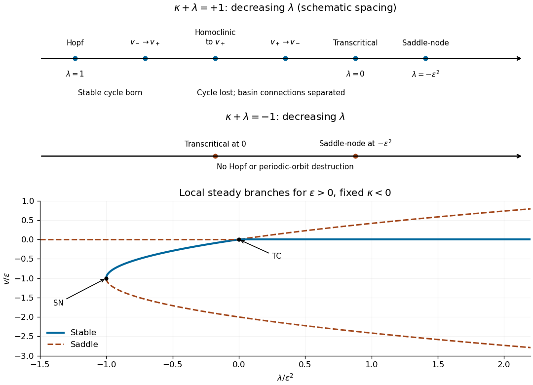
Bifurcation sequences along the two diagonal parameter lines after a small positive reflection-symmetry imperfection; arrows indicate decreasing lambda
. Details. Past exam of the mathematics course of the University of Cambridge 2004 iii Paper 60 1 e Solution by Codex 0 Created 2026-10-03 Updated 2026-10-14
Codex 0 Created 2026-10-03 Updated 2026-10-14Coordinate reflection in requires the th component to be odd in , and reflections in the other coordinates require it to be even in those coordinates. Thus no constant or quadratic terms are permitted. The only cubic monomials in component are and for . Coordinate permutations equate their coefficients in all components. After using the transverse linear eigenvalue as parameter, the normal form isThe remainder starts at fifth spatial order, together with parameter-dependent corrections such as . This is the cubic equivariants of the full cube symmetry group form. On a branch with equal nonzero absolute coordinates , respectively,Hence the three leading branch amplitudes are , and . Their generic nonzero denominators determine on which side the branches occur; existence alone does not make them stable.
Past exam of the mathematics course of the University of Cambridge 2004 iii Paper 60 1 d Solution by Codex 0 Created 2026-10-03 Updated 2026-10-14
Codex 0 Created 2026-10-03 Updated 2026-10-14Choose three representative vectors, with nonzero coordinate scale suppressed. Their stabilizer subgroups and fixed-point subspaces of a group action areHere exchanges the first two coordinates and exchanges the last two. On the first line the stabilizer subgroup is every signed permutation of the two zero coordinates; fixing it forces those coordinates to vanish. On the second line it exchanges the equal coordinates and independently reflects the zero coordinate, forcing . On the third line all coordinate permutations fix the vector, forcing .
The three subgroups have different orders and hence cannot be conjugate. Their group orbits contain respectively six face-axis, twelve edge-axis and eight vertex-axis directions. Each fixed-point subspace of a group action is one-dimensional, so the equivariant branching lemma guarantees three distinct symmetry types of bifurcating equilibria. The axial isotropy types of the full cube symmetry group are precisely these: a vector with several distinct nonzero absolute coordinate values has a separate freely variable coordinate block for each such value in the fixed-point subspace of a group action of its stabilizer subgroup, giving dimension greater than one.
Past exam of the mathematics course of the University of Cambridge 2004 iii Paper 60 1 c Solution by Codex 0 Created 2026-10-03 Updated 2026-10-14
Codex 0 Created 2026-10-03 Updated 2026-10-14Conjugating the coordinate reflection by the rotations supplies reflections in the other two coordinates. The quarter-turns, together with those reflections, also supply coordinate transpositions. Consequently the represented group consists of all signed permutation matrices, the full symmetry group of a cube of order .
Let be any real or complex matrix commuting with the group representation. Commutation with the three independent coordinate reflections forces all off-diagonal entries of to vanish. Commutation with the quarter-turn about the first axis equates its second and third diagonal entries, and the quarter-turn about the second axis equates its first and third entries. ThereforeFor completeness, if the complexified group representation had a proper invariant subspace, its orthogonal complement would be invariant too, since the generating matrices are unitary. The orthogonal projection onto that subspace would be a nonscalar commuting matrix, contradicting the calculation. Thus the complexification is irreducible, proving absolute irreducibility of the real group representation.
Pinned article: Introduction to the OurBigBook Project
Welcome to the OurBigBook Project! Our goal is to create the perfect publishing platform for STEM subjects, and get university-level students to write the best free STEM tutorials ever.
Everyone is welcome to create an account and play with the site: ourbigbook.com/go/register. We belive that students themselves can write amazing tutorials, but teachers are welcome too. You can write about anything you want, it doesn't have to be STEM or even educational. Silly test content is very welcome and you won't be penalized in any way. Just keep it legal!
Intro to OurBigBook
. Source. We have two killer features:
- topics: topics group articles by different users with the same title, e.g. here is the topic for the "Fundamental Theorem of Calculus" ourbigbook.com/go/topic/fundamental-theorem-of-calculusArticles of different users are sorted by upvote within each article page. This feature is a bit like:
- a Wikipedia where each user can have their own version of each article
- a Q&A website like Stack Overflow, where multiple people can give their views on a given topic, and the best ones are sorted by upvote. Except you don't need to wait for someone to ask first, and any topic goes, no matter how narrow or broad
This feature makes it possible for readers to find better explanations of any topic created by other writers. And it allows writers to create an explanation in a place that readers might actually find it.
Figure 1. Screenshot of the "Derivative" topic page. View it live at: ourbigbook.com/go/topic/derivativeVideo 2. OurBigBook Web topics demo. Source. - local editing: you can store all your personal knowledge base content locally in a plaintext markup format that can be edited locally and published either:This way you can be sure that even if OurBigBook.com were to go down one day (which we have no plans to do as it is quite cheap to host!), your content will still be perfectly readable as a static site.
- to OurBigBook.com to get awesome multi-user features like topics and likes
- as HTML files to a static website, which you can host yourself for free on many external providers like GitHub Pages, and remain in full control

Figure 2. You can publish local OurBigBook lightweight markup files to either OurBigBook.com or as a static website.
Figure 3. Visual Studio Code extension installation.
Figure 5. . You can also edit articles on the Web editor without installing anything locally. Video 3. Edit locally and publish demo. Source. This shows editing OurBigBook Markup and publishing it using the Visual Studio Code extension. 
- Infinitely deep tables of contents:




All our software is open source and hosted at: github.com/ourbigbook/ourbigbook
Further documentation can be found at: docs.ourbigbook.com
Feel free to reach our to us for any help or suggestions: docs.ourbigbook.com/#contact