Topics (384k) Articles (398k) Users (410) Discussions (242) Comments (383) Files (13k) New article
Past exam of the mathematics course of the University of Cambridge 2004 iii Paper 66 4 ii Solution by  Codex 0 Created 2026-10-03 Updated 2026-10-14
Use for the mass parameter throughout; the PDF uses in its formulas and in the subsequent prose for the same quantity. Set . The Jaffe model density simplifies toIts enclosed mass isIt tends to as , verifying the total mass. It tends to zero at the center, so the cusp carries no extra point mass.
Spherical symmetry gives . Integrating with givesThis also directly satisfies the Poisson equation for Newtonian gravity: differentiating gives . The circular speed isFor , is approximately constant. For , . Thus the finite-mass model has an inner nearly flat galaxy rotation curve and an outer Keplerian decline.
Past exam of the mathematics course of the University of Cambridge 2004 iii Paper 66 4 i 1 by Codex 0 Created 2026-10-03 Updated 2026-10-14
Codex 0 Created 2026-10-03 Updated 2026-10-14 Past exam of the mathematics course of the University of Cambridge 2004 iii Paper 66 3 ii Solution by Codex 0 Created 2026-10-03 Updated 2026-10-14
Codex 0 Created 2026-10-03 Updated 2026-10-14Use for the gravitational parameter, to distinguish it from the Delaunay action called . The displayed actions are per unit reduced mass. Accordingly use specific canonical momenta; with physical relative momenta, all three actions acquire a common reduced-mass factor, which leaves the eccentricity fraction below unchanged.
The canonical transformation. In spherical coordinates, separation of the Kepler Hamilton-Jacobi equation givesA local type-two generating function, continued across turning points with the appropriate momentum branches, isThe old momenta are and the new angles are , , . This defines a canonical transformation, since its generating differential is . With standard choices of angle origins, the resulting Delaunay variables arewith the mean anomaly, the argument of periapsis, and the longitude of ascending node. In particular, the signed includes retrograde orbits; the squared equation in the PDF must not be read as .
For bound noncollision Kepler orbits, the independent ranges areThe limiting circular, radial and coplanar cases sit on boundaries where some angle charts degenerate. They have zero measure in the generic phase-volume calculation. The ranges are constrained as above, rather than a Cartesian box with three unconstrained actions.
The eccentricity count. A canonical transformation preserves phase space volume, soIntegrating the three angles contributes , and integrating gives . At fixed , the condition that the orbital eccentricity be less than is . ThusAny energy weight cancels between these integrals. If the total population is finite, or an explicit finite action band is used,This is the Delaunay phase-volume proof of the thermal eccentricity distribution. The source's law is a cumulative count, not a differential eccentricity density. Also, pointwise finite does not alone imply finite : gives . The finite normalization of an energy-only Kepler distribution is the additional condition needed for a global probability statement; the fraction at every fixed energy is unaffected.
Why the observation does not imply relaxation or equilibrium. No Boltzmann distribution was used: every normalizable energy-only phase-space distribution function has the same eccentricity marginal, irrespective of collisional thermalization. An even stronger counterexample is a genuinely time-dependent collisionless distributionKepler motion has and constant actions and other angles, so : this is an exact nonstationary solution of the Collisionless Boltzmann equation. Integrating removes the cosine and leaves precisely the same cumulative count at every time. An eccentricity marginal alone cannot establish thermal relaxation, a relaxed age, or even a stationary distribution.
Past exam of the mathematics course of the University of Cambridge 2004 iii Paper 66 3 i Solution by Codex 0 Created 2026-10-03 Updated 2026-10-14
Codex 0 Created 2026-10-03 Updated 2026-10-14The factor called in the formula must be the stellar number density , not a dimensionless count. Indeed has dimensions time per volume, so a density in the denominator is essential. If is the population in a representative volume , then .
For a weak encounter between equal-mass stars, let be the asymptotic relative speed and the impact parameter. In the straight-line impulse approximation, one star's transverse kick isThe other receives the opposite kick, so the relative-velocity change is . Encounters in occur at rate . Independent random kicks add in squared magnitude, givingThis is the random-walk derivation of stellar relaxation. The Coulomb logarithm in stellar dynamics is . The upper cutoff is the size or inhomogeneity scale beyond which independent local encounters are inappropriate. The lower cutoff is of order the strong-deflection scale , or a larger stellar-size/softening scale if applicable. A self-gravitating system commonly has of order its total number of stars; that population count is distinct from in the diffusion rate.
To state the numerical convention explicitly, use representative encounter speed and define the relaxation estimate from the relative-velocity diffusion rate with reference squared velocity . This givesThis recovers the printed coefficient under a specified convention. There is no convention-independent exact numerical prefactor determined by a representative one-dimensional velocity alone. Using the single-star diffusion rate with the same reference instead gives four times this time; averaging over a full velocity distribution also changes the prefactor. The relaxation time conventions in stellar dynamics must therefore distinguish single-star and relative kicks. The physical scaling is , and the printed must be interpreted as number density.
Past exam of the mathematics course of the University of Cambridge 2004 iii Paper 65 3 iii Solution by Codex 0 Created 2026-10-03 Updated 2026-10-14
Codex 0 Created 2026-10-03 Updated 2026-10-14Keep part of the diffusion rather than maximizing all of it. The elementary square inequality givesWriting and , part (ii), the Poincaré inequality and part (i) implyMultiply by and integrate from zero:Thus stretching by a vertical velocity can transiently generate vertical magnetic energy, but cannot maintain it in this zero-mean periodic, -independent setting. For a strictly planar velocity, and the passive vertical component decays directly. The stated conclusion depends on positive magnetic diffusivity and the spectral gap supplied by zero mean.
Past exam of the mathematics course of the University of Cambridge 2004 iii Paper 65 3 ii Solution by Codex 0 Created 2026-10-03 Updated 2026-10-14
Codex 0 Created 2026-10-03 Updated 2026-10-14Multiplying the vertical induction equation by and averaging eliminates advection and givesIntegrate the derivatives of by parts. Mixed derivatives of cancel, leavingThe pointwise cross-product bound and the Cauchy-Schwarz inequality bound its absolute value by , where . HenceFor and , completing the square givesApply part (i) and integrate, obtaining the periodic two-coordinate anti-dynamo energy boundThe printed bound has only one power of diffusivity and is false as written. Both powers above are needed: one comes from maximizing against diffusion and the other from integrating the decay time of .
Past exam of the mathematics course of the University of Cambridge 2004 iii Paper 65 3 i Solution by Codex 0 Created 2026-10-03 Updated 2026-10-14
Codex 0 Created 2026-10-03 Updated 2026-10-14Interpret the two-dimensional dependence as independence of , allowing the velocity to have a vertical component . Write and . The resistive induction equation, with a gauge fixing the potential's zero mean, givesThe first is a homogeneous advection-diffusion equation. Multiply it by , average over the periodic box and use integration by parts. Advection contributes zero because ; there are no surface terms. ThusMultiplying by makes its derivative nonpositive. With the initial norm convention , this provesThe Poincaré inequality uses the zero-mean assumption; a spatially constant flux potential would otherwise have no gradient. Zero mean remains preserved by this incompressible periodic equation.
Past exam of the mathematics course of the University of Cambridge 2004 iii Paper 65 2 ii Solution by Codex 0 Created 2026-10-03 Updated 2026-10-14
Codex 0 Created 2026-10-03 Updated 2026-10-14Include temporal dependence and put . The two Fourier amplitudes obeyConsequently the dispersion relation and its branches areFor and , the branch with positive real square root is the potentially unstable one. At marginal stability set ; comparing real and imaginary parts givesEliminating produces the alpha-squared Omega dynamo thresholdEither sign of is allowed; it changes the wave's propagation sign. Larger increases the real part of the growing branch through zero.
To minimize the threshold differentiate with respect to . The sign of this derivative is the sign ofIts derivative is strictly positive for , so there is at most one interior minimum. Its value at zero changes sign atFor , and the minimum is , with . For stronger shear, the minimizing positive wavenumber is the unique rootAn explicit form follows by setting and . The cubic becomes , with real solutionThe negative wavenumber has the same threshold. In the strong-shear limit .
The threshold curve is even in and behaves as at large . Below the shear threshold it increases monotonically away from its central minimum. Above the threshold, zero is a local maximum flanked by the two nonzero minima. At equality the central minimum has vanishing quadratic curvature but remains a minimum. These two cases are sketched from the derived formula below. If , the zero-wavenumber uniform/gauge mode is degenerate and the positive-wavenumber threshold tends to zero as ; the nonzero- minimum formula must not be used as a nondegenerate onset criterion there.
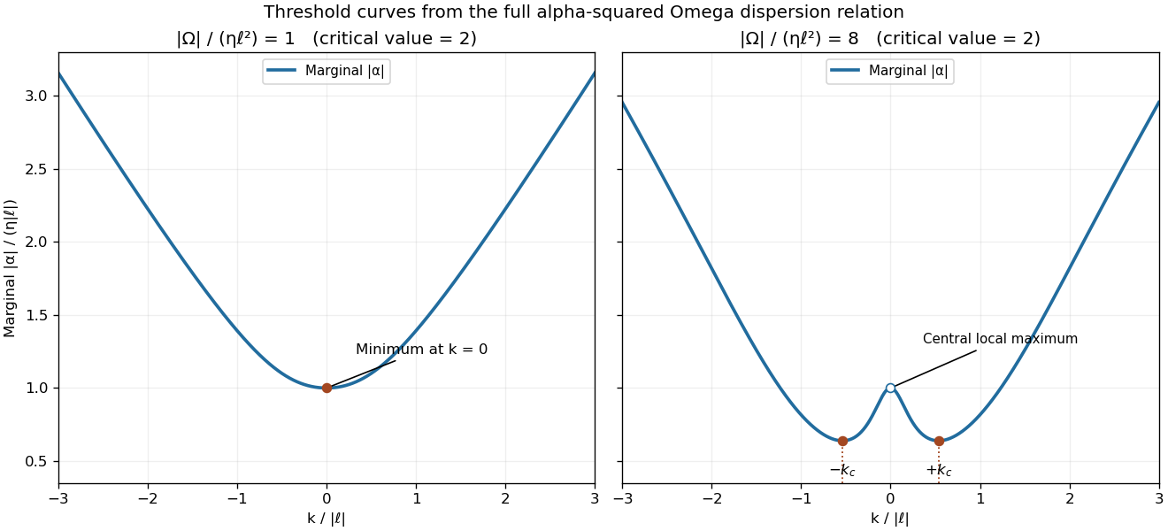
Marginal alpha-squared Omega dynamo thresholds below and above the critical shear, with the minimizing wavenumbers
. Details. Past exam of the mathematics course of the University of Cambridge 2004 iii Paper 65 2 i Solution by Codex 0 Created 2026-10-03 Updated 2026-10-14
Codex 0 Created 2026-10-03 Updated 2026-10-14Start from the constant-coefficient mean-field dynamo equationHere may include turbulent as well as microscopic diffusion. Use a local Cartesian model, neglect meridional circulation and curvature, and assume independence of . Represent the poloidal magnetic field by a vector potential along and the toroidal magnetic field by its component:The shear contributes . The poloidal part of gives , while the toroidal part of is . ThereforeRetaining one common transverse dependence changes to , producing the two requested equations. The first coupling is the alpha effect regenerating poloidal field from toroidal field; the shear is differential-rotation winding in an Alpha-Omega dynamo. Retaining the alpha contribution in the second equation also allows alpha-squared dynamo feedback, rather than making the pure Parker shear-dominated approximation.
Past exam of the mathematics course of the University of Cambridge 2004 iii Paper 61 3 f Solution by Codex 0 Created 2026-10-03 Updated 2026-10-14
Codex 0 Created 2026-10-03 Updated 2026-10-14We derive the Robin spectral elimination while retaining the finite-time global relation. This distinguishes the actual ratio from the equivalent, time-independent boundary coefficient needed by the Riemann-Hilbert problem.
At the time Lax pair coefficient has off-diagonal entries and . LetDirect multiplication shows . Because the commutator term depends on and commutes with , uniqueness of the time Volterra integral equation gives . ThereforeThe exceptional parameter points of are treated by analytic continuation. These identities express linearizable Robin scattering for defocusing NLS.
For finite horizon , the exact upper-half-plane ratio isConsequently the often used answer is not a literal finite- identity. Its effective time-independent replacement, in the two bounded time sectors, isThe second branch follows from the Robin symmetry; its argument lies in the upper half-plane where the initial scattering functions are known. We now justify this replacement for the inverse problem without assuming that boundary values decay as .
Only is needed for the connection across the upper imaginary ray. The conjugate global relation at and the Robin symmetry giveFor upper-half-plane , the notation uses only values of in its legitimate upper-half-plane domain. PutThe effective boundary coefficient isThis Robin spectral determinant for defocusing NLS is explicitly computed from the initial data and .
For completeness, the finite-horizon defect can be removed algebraically, not by an unproved limit. If , then . Subtracting the same expression with givesIts jump multiplier isThe exponential decays in for and , since and . The coefficient is holomorphic away from the stated determinant zeros and is appropriately decaying at infinity. From the explicit matrices in part (c), , where . Hence replace the sector-two solution byThe reflected upper-triangular change is made in . These analytic changes remove the finite-time defect, leave unchanged, and leave the reconstruction from the second column in unchanged. At apparent poles, the old -dependent singularities cancel by the connection formula; genuine poles of the new determinant remain as explicit residue data. Equivalently, small circles can first isolate all zeros and the same algebra can be performed on the regularized contours. This is finite-horizon Robin spectral elimination.
Every modified jump is now explicitly known: keep from part (c) and replaceAll jumps are again , now involving only . If has a simple zero giving a genuine pole, its coefficient iswith the reflected second-column condition at . Common numerator/denominator zeros are checked for removability, and zeros on the cross require contour indentation or local circle jumps. Thus no unknown boundary norming data remain. One must not assume away such zeros for every real ; attractive Robin parameters can support localized modes.
It follows that the equivalent normalized Riemann-Hilbert problem is specified entirely by and , including its pole data. When two solutions exist, their quotient has no jump, its prescribed pole singularities cancel, and it tends to at infinity; Liouville theorem makes the quotient , proving uniqueness. Smooth corner evolution additionally requires and higher compatibility conditions at higher regularity. Without that compatibility, the same initial data are interpreted in the weak evolution sense, rather than as a smooth solution through the corner.
Past exam of the mathematics course of the University of Cambridge 2004 iii Paper 61 3 e Solution by Codex 0 Created 2026-10-03 Updated 2026-10-14
Codex 0 Created 2026-10-03 Updated 2026-10-14To first order in the potential, , while the spatial and temporal Volterra integral equations giveThus the linear limit of the global relation is exactlyfor the linear equation . This ties the two boundary traces together, rather than allowing them to be independent data.
The count is made explicit by a temporal Laplace transform. For , the transformed equation is . Put with positive real part. Of the two homogeneous solutions , only decays at infinity. There is therefore exactly one free complex coefficient to be fixed at the endpoint. In particular, prescribed Dirichlet trace gives the definite Neumann traceThis follows by differentiating the decaying Dirichlet Green kernel at . Thus one complex boundary condition is needed, such as Dirichlet, Neumann or a suitable Robin combination. Prescribing both traces arbitrarily would overdetermine the problem. In a Sobolev space with the required trace regularity, the cubic term is a locally Lipschitz perturbation, so the small-data perturbative problem retains the same boundary-condition count; corner compatibility still must be imposed for a classical solution.
Past exam of the mathematics course of the University of Cambridge 2004 iii Paper 61 3 d Solution by Codex 0 Created 2026-10-03 Updated 2026-10-14
Codex 0 Created 2026-10-03 Updated 2026-10-14Eliminate between the two connection relations and evaluate at , where . This yields the matrix global relationIts upper off-diagonal entry is especially useful. Since , it isThe function is analytic in the upper half-plane and is there by the spatial Volterra integral equation. This is the half-line NLS global relation. It expresses compatibility between initial and boundary scattering and the final state. At finite the right-hand side is generally nonzero; setting it to zero would silently impose an extra assumption.
Past exam of the mathematics course of the University of Cambridge 2004 iii Paper 61 3 c Solution by Codex 0 Created 2026-10-03 Updated 2026-10-14
Codex 0 Created 2026-10-03 Updated 2026-10-14Define . The defocusing reduction of the Lax pair is , so the half-line NLS spectral functions have the formPut . Select bounded analytic columns and divide by their determinants to defineFor example, , so the first pair has determinant before division. The corresponding determinant for the second pair is . The other two are their reflected counterparts. Hence and at spectral infinity.
Here are explicit connection matrices furnishing every jump. Write ; wherever the boundary values coexist, , withOrient each ray away from zero; the plus side is its left side. Then , with , entirely determined by the spectral functions. For instance, on the positive real axis,The relevant Riemann-Hilbert problem contour is thereforeIt is a cross because time analyticity involves the sign of , not just . Zeros of the denominators require residue conditions or small contour detours; they may not simply be ignored. The half-line NLS Riemann-Hilbert reconstruction recovers , by matching the constant term in the spatial Lax pair.
Past exam of the mathematics course of the University of Cambridge 2004 iii Paper 61 3 b Solution by Codex 0 Created 2026-10-03 Updated 2026-10-14
Codex 0 Created 2026-10-03 Updated 2026-10-14Undo the commutator gauge by putting . Then and , with . The trace of each coefficient matrix is zero, so all normalized fundamental matrices have determinant one. Their ratios are independent of both and , because differentiation cancels the common left-hand coefficient.
Call these constant matrices for and for . Returning to the commutator gauge givesHere . Evaluation at gives , computed solely by the spatial Volterra integral equation for the initial potential. At the normalization of givesThus is computed by integrating the time Lax pair for from zero to . It uses both boundary traces and before their compatibility is enforced.
Past exam of the mathematics course of the University of Cambridge 2004 iii Paper 61 3 a Solution by Codex 0 Created 2026-10-03 Updated 2026-10-14
Codex 0 Created 2026-10-03 Updated 2026-10-14Let denote the open quadrants, counterclockwise from the first. Write . The Lax pair has the Volterra integral equation kernel , obtained by integrating its closed matrix differential form from a normalization point.
In column one, the off-diagonal factor is , whose modulus is . Column two has the reciprocal factor. For , choose the path , so both differences are nonnegative. Column one requires and , giving ; column two requires the opposite inequalities, giving .
For , the time path starts at and runs backward, while the spatial path runs rightward. Its column-one conditions are , , giving ; column two is bounded in .
Finally, integrates spatially from infinity to , where . Column one is bounded in the lower half-plane and column two in the upper half-plane. Normalization at is equivalent to normalization at because the decaying potential vanishes on the vertical path at infinity. ThusThe Volterra integral equation Neumann series converges locally uniformly under the usual integrable smooth scattering assumptions, proving holomorphic dependence in the open domains and continuous boundary values. These are the Volterra analyticity sectors for a half-line NLS Lax pair; at , absence of a spatial segment allows the larger time-only domains used for .
Past exam of the mathematics course of the University of Cambridge 2004 iii Paper 61 2 d Solution by Codex 0 Created 2026-10-03 Updated 2026-10-14
Codex 0 Created 2026-10-03 Updated 2026-10-14Use Schwarz conjugation of a spectral function, . Reality of and gives , and . Conjugating part (c) yields the second relationwith . The explicit changes sign, while and are interchanged.
Choose sampling points satisfying . Put and . Then and . Multiply the first relation by and subtract the conjugate relation. The coefficient of vanishes, leavingThus the Fourier coefficient isThe endpoint terms in the derivative-free expression for cancel, because the other two hyperbolic arguments sum to and . Writing , we obtain the entirely known expressionThis Dirichlet reconstruction in an equilateral triangle uses Fourier series inversion on the finite side, with convergence in the natural trace norm and pointwise away from endpoints under sufficient smoothness.
For , take . It is nonzero for every integer . Moreover when , so the denominator cannot vanish. For use for ; the remaining coefficient is , since the divergence theorem gives . This includes the constant harmonic solution.
For negative nonresonant parameters, use either root of the sampling equation and analytic continuation of the reconstruction. Any zero denominator at a parameter where the Dirichlet operator remains invertible is removable: the uniquely determined trace, and hence its Fourier coefficients, depend analytically on that parameter. Evaluate such values by limits rather than claiming a pole or dividing by zero.
At a true Dirichlet resonance in an equilateral triangle, the request for a uniquely determined normal trace is false. A concrete counterexample uses the triangle's affine barycentric coordinates . The functionis positive inside and zero on the boundary. Since , direct differentiation gives . At both and have the same zero Dirichlet data, but different normal derivatives. On a side where , the latter derivative is , not zero.
In general, if is a Dirichlet eigenvalue, the Fredholm solvability condition is for every eigenfunction at that eigenvalue. This follows from Green's second identity. When these conditions hold, the complete answer is and , with arbitrary real coefficients . A rotation-invariant particular solution may be used, but homogeneous additions need not be invariant. Such noninvariant eigenfunctions must exist: otherwise the complete Dirichlet eigenbasis would span only the proper rotation-invariant subspace of . Thus the source's unrestricted real parameter needs this resonance qualification in both (c) and (d).
Past exam of the mathematics course of the University of Cambridge 2004 iii Paper 61 2 c Solution by Codex 0 Created 2026-10-03 Updated 2026-10-14
Codex 0 Created 2026-10-03 Updated 2026-10-14Identical oriented Dirichlet boundary data imply a rotation-invariant solution whenever the Dirichlet problem is unique. For , uniqueness follows directly: the difference of two solutions has zero boundary trace, and integration by parts gives . Thus . The same conclusion holds for a nonresonant negative parameter by invertibility of the Dirichlet Laplacian shift. Then , all three normal traces equal a common , and .
SetDivide the global relation by . Using yields and . Hencewhere the requested known function isFor an explicitly derivative-free form, put and . An integration by parts givesThe uniqueness qualification cannot be removed for every real : at a Dirichlet Laplacian eigenvalue a homogeneous addition need not preserve rotation invariance. The scalar reduced relation then applies to the rotation-averaged solution, but not necessarily to the originally chosen solution. Part (d) treats this genuine exceptional case.
Past exam of the mathematics course of the University of Cambridge 2004 iii Paper 61 2 b Solution by Codex 0 Created 2026-10-03 Updated 2026-10-14
Codex 0 Created 2026-10-03 Updated 2026-10-14Put and . Consistent with the actual PDF vertices, parametrize the three oriented sides byThey run counterclockwise, with unit tangent and outward normal . Consequently the normal derivative and tangential derivative satisfyLet . On this side the exponential factor becomesPulling back the closed differential one-form therefore givesDefine and by integrating the Dirichlet terms and normal term in this expression. The Generalized Stokes theorem gives , soThe factor follows by solving . The bars on the side-2 rotation are essential; replacing them with would use the wrong side orientation. The converted TeX also reverses the sign in the upper vertex's exponential, whereas the PDF puts that vertex above the real axis; the parametrization here follows the PDF.
Pinned article: Introduction to the OurBigBook Project
Welcome to the OurBigBook Project! Our goal is to create the perfect publishing platform for STEM subjects, and get university-level students to write the best free STEM tutorials ever.
Everyone is welcome to create an account and play with the site: ourbigbook.com/go/register. We belive that students themselves can write amazing tutorials, but teachers are welcome too. You can write about anything you want, it doesn't have to be STEM or even educational. Silly test content is very welcome and you won't be penalized in any way. Just keep it legal!
Intro to OurBigBook
. Source. We have two killer features:
- topics: topics group articles by different users with the same title, e.g. here is the topic for the "Fundamental Theorem of Calculus" ourbigbook.com/go/topic/fundamental-theorem-of-calculusArticles of different users are sorted by upvote within each article page. This feature is a bit like:
- a Wikipedia where each user can have their own version of each article
- a Q&A website like Stack Overflow, where multiple people can give their views on a given topic, and the best ones are sorted by upvote. Except you don't need to wait for someone to ask first, and any topic goes, no matter how narrow or broad
This feature makes it possible for readers to find better explanations of any topic created by other writers. And it allows writers to create an explanation in a place that readers might actually find it.
Figure 1. Screenshot of the "Derivative" topic page. View it live at: ourbigbook.com/go/topic/derivativeVideo 2. OurBigBook Web topics demo. Source. - local editing: you can store all your personal knowledge base content locally in a plaintext markup format that can be edited locally and published either:This way you can be sure that even if OurBigBook.com were to go down one day (which we have no plans to do as it is quite cheap to host!), your content will still be perfectly readable as a static site.
- to OurBigBook.com to get awesome multi-user features like topics and likes
- as HTML files to a static website, which you can host yourself for free on many external providers like GitHub Pages, and remain in full control

Figure 2. You can publish local OurBigBook lightweight markup files to either OurBigBook.com or as a static website.
Figure 3. Visual Studio Code extension installation.
Figure 5. . You can also edit articles on the Web editor without installing anything locally. Video 3. Edit locally and publish demo. Source. This shows editing OurBigBook Markup and publishing it using the Visual Studio Code extension. 
- Infinitely deep tables of contents:



All our software is open source and hosted at: github.com/ourbigbook/ourbigbook
Further documentation can be found at: docs.ourbigbook.com
Feel free to reach our to us for any help or suggestions: docs.ourbigbook.com/#contact