Topics (384k) Articles (398k) Users (410) Discussions (242) Comments (383) Files (13k) New article
Past exam of the mathematics course of the University of Cambridge 2004 iii Paper 53 3 3 Solution by  Codex 0 Created 2026-10-03 Updated 2026-10-14
Assume the three physical phase-flip channels act independently, with the same probability on each qubit, and encoding, recovery and decoding are ideal. Zero or one physical error is corrected. HenceThe probability of an uncorrectable two- or three-site error is .
One must also choose the logical convention consistently with the output phase error specified here. The usual phase-flip repetition code with codewords and has residual operator after two or three physical errors: their error syndrome equals that of the complementary zero- or one-error pattern. This operator exchanges those codewords, so plain inverse encoding would give logical , not .
To obtain the stated logical phase-flip convention, use the logical Hadamard convention for a phase-flip repetition code. Put a logical Hadamard gate before that encoding and after its decoding. The encoded state iswhere the plus and minus states in these codewords are the real Hadamard basis states. The uncorrectable exchange is now conjugated to . With that convention the decoded density operator and its trace distance are exactlyFor , , so coding reduces the trace distance. The displayed recovery probability means success of correction as a quantum operation on an arbitrary unknown input. If the particular input is a eigenstate, even the logical phase-error branch represents the same physical state, and the probability of recovering that particular state is one.
Independence is an extra noise assumption needed for the numerical probability. If all three physical qubits flip together with probability , each marginal still has the given phase-flip channel, but the logical failure probability is , not . More generally, for a classical joint phase-error distribution with a random number of flips, and ; the same decoded mixture holds in the stated logical convention. Thus marginal error probabilities alone do not determine the requested recovery probability. A complex environment overlap likewise requires the coherent rotation to be retained or separately compensated before this stochastic phase-error analysis applies.
Past exam of the mathematics course of the University of Cambridge 2004 iii Paper 53 3 2 Solution by Codex 0 Created 2026-10-03 Updated 2026-10-14
Codex 0 Created 2026-10-03 Updated 2026-10-14Subtract the two density operators. The difference is Hermitian with zero diagonal and off-diagonal entry . A matrix has eigenvalues , because its square is . Its two singular values are therefore both . By the definition of the trace norm,For the intended real-overlap phase-flip channel, , givingThis vanishes for a computational basis state, since a phase flip then changes only an unobservable global phase. Its largest value at fixed is , attained when . The general formula remains correct even when the probabilistic premise of part 1 fails.
Past exam of the mathematics course of the University of Cambridge 2004 iii Paper 53 3 1 Solution by Codex 0 Created 2026-10-03 Updated 2026-10-14
Codex 0 Created 2026-10-03 Updated 2026-10-14Let . The joint state after the environment interaction is . Taking its partial trace over the environment gives the exact reduced density operatorThe conjugate in the upper off-diagonal entry follows from tracing . Normalization of the environment states and the Cauchy-Schwarz inequality imply .
For comparison, a phase-flip channel sends to , multiplying its off-diagonal entries by the real number . Consequently the claimed representation is valid, for a general input, provided the environment overlap is real, withThis is a genuine probability between zero and one. The environment maps printed in the question do not themselves imply that is real. For example, choose , so , and take . The qubit becomes , whose imaginary off-diagonal entries cannot come from any probabilistic mixture of and . These environment maps are a valid isometry and can be extended to a unitary interaction, so this is an actual counterexample to the unrestricted premise.
The general complex environment overlap in qubit dephasing has an exact corrected description. Write , , and let . ThenAt , choose any phase. The dephasing channel includes both random phase errors and, when the overlap is complex, a coherent diagonal rotation. The subsequent probability formulas use the intended real-overlap phase-flip model.
Past exam of the mathematics course of the University of Cambridge 2004 iii Paper 53 2 2 Solution by Codex 0 Created 2026-10-03 Updated 2026-10-14
Codex 0 Created 2026-10-03 Updated 2026-10-14The first Hadamard transform prepares a uniform superposition in the first register while the second stays zero. The Boolean quantum oracle, now with an -bit output register and bitwise addition, therefore givesThis state is normalized because distinct labels are orthogonal, even when their oracle outputs coincide. Addition in the oracle is bitwise exclusive-or, making the oracle reversible; replacing the first register by would not define a unitary gate for a two-to-one function.
For the later recovery steps we use the intended nonzero hidden-period promise . Then two-to-one behavior and force each fibre to be exactly . The printed allowance does not explicitly exclude zero. If zero were allowed without a nonzero-period promise, the displayed identity would hold trivially for every function and would not specify Simon's problem. That distinction is addressed again in the query count.
Past exam of the mathematics course of the University of Cambridge 2004 iii Paper 53 2 1 Solution by Codex 0 Created 2026-10-03 Updated 2026-10-14
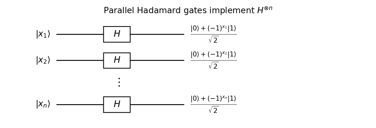
Codex 0 Created 2026-10-03 Updated 2026-10-14Apply one Hadamard gate independently to each qubit. These gates act in parallel, so the quantum circuit implements with gates and depth one.
Parallel Hadamard gates implementing the binary Fourier transform
. Details. For a computational basis state, factorization givesThe exponent is the dot product over the finite field , because multiplying the separate signs adds their exponents modulo two. This is the Walsh-Hadamard transform, equivalently the quantum Fourier transform on the finite Abelian group .
In particular, the all-zero input becomes the uniform coherent superposition . It is a useful initial operation because an oracle can then act on all amplitudes in one call, and subsequent interference can reveal a global property. Measurement alone does not read all function values: the later interference step is what turns the preparation into an algorithmic advantage.
Past exam of the mathematics course of the University of Cambridge 2004 iii Paper 50 3 b Solution by Codex 0 Created 2026-10-03 Updated 2026-10-14
Codex 0 Created 2026-10-03 Updated 2026-10-14The same Super-Poincaré algebra gives the operator identityFor a normalized physical state in a positive-norm Hilbert space,An unbroken supersymmetric vacuum must be annihilated by every supercharge and its adjoint, hence has zero energy. Conversely, zero expectation of this positive sum forces each norm separately to vanish. Therefore a vacuum with strictly positive energy necessarily breaks supersymmetry. For an infinite-volume field theory the corresponding statement is about vacuum energy density, obtained with an appropriate finite-volume regulator. The zero of energy is fixed by the algebra; it cannot be arbitrarily shifted while preserving this identity. This is the global-supersymmetry result and does not assert positivity of the general local-supergravity scalar potential.
Past exam of the mathematics course of the University of Cambridge 2004 iii Paper 50 3 a Solution by Codex 0 Created 2026-10-03 Updated 2026-10-14
Codex 0 Created 2026-10-03 Updated 2026-10-14For global four-dimensional supersymmetry, useLet be fermion parity. On a finite one-particle supermultiplet at fixed positive-energy momentum, the supercharges act within the multiplet and . Cyclicity of the finite-dimensional trace givesThus the trace with of every displayed diagonal anticommutator vanishes. Summing the two components, , soSince , this proves , for both massive and massless one-particle multiplets. The restriction matters: a zero-momentum supersymmetric vacuum singlet, annihilated by every supercharge, need not contain a fermionic partner. The algebra does not imply equal counts for such a trivial zero-energy representation or for an arbitrary unregulated infinite-dimensional trace.
Past exam of the mathematics course of the University of Cambridge 2004 iii Paper 50 1 d Solution by Codex 0 Created 2026-10-03 Updated 2026-10-14
Codex 0 Created 2026-10-03 Updated 2026-10-14Both Kaluza-Klein theory and the brane-world scenario use a higher-dimensional bulk. Ordinary Kaluza–Klein matter propagates in the compact directions, producing observable massive towers; absence of weak-scale charged modes requires roughly , or , and traditional constructions often take Planck-size radii. Brane-world matter is localized while gravity explores the bulk, so large flat dimensions can reach the submillimetre order of magnitude discussed in the 2004 setting. For flat dimensions, . These are model-dependent scales, not universal maxima: warped gravity-localizing models can have a noncompact extra dimension. The historical large-flat-dimension mechanism is described in arxiv.org/abs/hep-ph/9803315.
Past exam of the mathematics course of the University of Cambridge 2004 iii Paper 50 1 c Solution by Codex 0 Created 2026-10-03 Updated 2026-10-14
Codex 0 Created 2026-10-03 Updated 2026-10-14In a supersymmetric Higgs mechanism, an internal gauge symmetry breaks while supersymmetry can remain unbroken. A massless vector multiplet absorbs a chiral multiplet and becomes a massive multiplet with spins : the gauge boson acquires its longitudinal particle polarization from the Goldstone mode. In the super-Higgs mechanism, local supersymmetry itself breaks: the spin- gravitino absorbs the spin- goldstino, gaining two longitudinal polarizations and becoming massive. With only global supersymmetry breaking, the goldstino instead remains a physical massless fermion.
Past exam of the mathematics course of the University of Cambridge 2004 iii Paper 50 1 b Solution by Codex 0 Created 2026-10-03 Updated 2026-10-14
Codex 0 Created 2026-10-03 Updated 2026-10-14TeV-scale softly broken supersymmetry addresses the technical hierarchy problem: equal bosonic and fermionic couplings cancel quadratic ultraviolet contributions to the Higgs mass. Soft mass splittings leave corrections of order , so a weak-scale soft spectrum protects the weak scale against a much higher cutoff. Unbroken four-dimensional extended supersymmetry is incompatible with the observed complex chiral gauge spectrum: charged hypermultiplets contain conjugate representations, while vector multiplets have real adjoint matter. It must therefore be broken to at most before reproducing low-energy Standard Model chirality.
Past exam of the mathematics course of the University of Cambridge 2004 iii Paper 50 1 a Solution by Codex 0 Created 2026-10-03 Updated 2026-10-14
Codex 0 Created 2026-10-03 Updated 2026-10-14Positive-energy one-particle Poincaré group representations have labels for , and for finite-helicity massless states; individual massive polarizations add . An massive supermultiplet is labelled by mass and superspin , with constituent labelsA massless supermultiplet has constituent labelsA CPT completion of a supermultiplet additionally supplies , with conjugated internal charges where applicable. Constituent spins/helicities are the labels here, not counts of polarizations.
Past exam of the mathematics course of the University of Cambridge 2004 iii Paper 47 2 c Solution by Codex 0 Created 2026-10-03 Updated 2026-10-14
Codex 0 Created 2026-10-03 Updated 2026-10-14Use and . Its cubic and quartic Yang-Mills self-interactions areAntisymmetry of the Lie algebra structure constants lets the cubic expression also be written as .
The cubic vertex has three fields and one derivative, corresponding to in part (b). The quartic vertex has four fields and no derivatives, corresponding to . Their dimensions areWith both types present, the same Feynman diagram counting givesIn four dimensions both couplings are dimensionless, and the degree is bounded independently of vertex count. Gauge symmetry, implemented consistently after gauge fixing, restricts the ultraviolet counterterms to the allowed renormalizable gauge-invariant and gauge fixing/ghost structures. Thus the counting is consistent with perturbative renormalizability of ordinary four-dimensional Yang-Mills theory.
In six dimensions and , giving . Increasing the vertex count permits new divergent momentum structures and higher-dimensional operators without a finite closed list of renormalization parameters. Ordinary Yang-Mills theory is therefore power-counting renormalizable in four dimensions and nonrenormalizable in six dimensions. It can still be used in six dimensions as an effective field theory with a cutoff and higher-operator expansion; this conclusion concerns the usual perturbative theory.
Past exam of the mathematics course of the University of Cambridge 2004 iii Paper 47 2 b Solution by Codex 0 Created 2026-10-03 Updated 2026-10-14
Codex 0 Created 2026-10-03 Updated 2026-10-14The kinetic normalization fixes , since a derivative has mass dimension one and the Lagrangian density has dimension . Every differentiated field is still a field insertion. Hence the interaction has legs, not just , and its vertex contains a homogeneous polynomial of degree in the attached momenta. Its coupling dimension isFor a connected Feynman diagram of this vertex type,The superficial momentum degree is now . Eliminating and givesso derivative-interaction scalar power counting yieldsThe same counting applies to tensor components with quantum field theory propagators scaling as ; contractions, identities and cancellations can lower the actual degree. A coupling of negative mass dimension lets the superficial degree increase with the number of vertices, explaining the need for progressively higher-dimensional counterterms in a perturbative effective field theory.
Past exam of the mathematics course of the University of Cambridge 2004 iii Paper 47 2 a Solution by Codex 0 Created 2026-10-03 Updated 2026-10-14
Codex 0 Created 2026-10-03 Updated 2026-10-14Let a connected amputated one-particle-irreducible Feynman diagram have loops, internal lines, quartic vertices and external legs. Each loop integration contributes four momentum powers, each scalar propagator removes two, and the interaction adds none. Thus its superficial degree of divergence is . Counting half-edges and independent loops givesThis is simultaneous large-momentum scaling of the whole Feynman diagram. It need not describe every subregion of loop-momentum space.
For a concrete counterexample, start with a six-point triangle of three quartic vertices, with two external legs at each vertex. Insert a one-loop tadpole diagram self-energy in one internal line. The resulting Feynman diagram has , , , , and . It is still one-particle irreducible: each edge around the triangle has an alternative route, and cutting the tadpole loop does not disconnect the Feynman diagram. Nevertheless the tadpole subgraph diverges when its loop momentum tends to infinity while the triangle momentum is held fixed. In massive theory the divergent mass insertion is nonzero. This demonstrates that a superficially convergent graph can have a divergent subgraph.
Write renormalized perturbation theory withThe last term is a field-independent vacuum counterterm, needed if vacuum energies are retained. A normalized correlation functional removes that sector. The free quantum field theory propagator is ; interaction and counterterm insertions useUsual momentum-conservation delta functions accompany the vertices. The coefficients depend on the regulator and renormalization conditions and are expanded order by order in the renormalized coupling.
The reason this list closes is locality of ultraviolet subtraction. After divergent proper subgraphs have been subtracted recursively, the remaining overall divergent part is a polynomial in external momenta of degree at most . For , , Lorentz symmetry allows only a constant and a term, supplied by the mass and wavefunction counterterms. For , , only the constant quartic counterterm is needed. Odd-point terms vanish by the field's symmetry. For , the overall degree is negative and there is no new overall counterterm after subdivergences have been removed. Vacuum graphs are handled separately.
Counterterm insertions subtract each subgraph's local divergence, including overlapping subgraphs, and then the overall divergence. At each perturbative order the regulated sum has a finite ultraviolet limit for renormalized correlation functions at suitable nonexceptional momenta. This is why superficial power counting of every relevant subgraph determines the allowed counterterms, even though it does not alone establish that a bare Feynman diagram diverges or converges. Possible infrared or on-shell singularities are a separate issue; ultraviolet renormalization is not a promise of finiteness in every kinematic limit.
Past exam of the mathematics course of the University of Cambridge 2004 iii Paper 46 2 e Solution by Codex 0 Created 2026-10-03 Updated 2026-10-14
Codex 0 Created 2026-10-03 Updated 2026-10-14Within a finite blocking step, is generally analytic near the critical couplings because only finitely many microscopic variables have been summed. If its regular contribution can be removed by the analytic subtraction of an inhomogeneous renormalization recursion, derivatives of that background are nonsingular. The critical powers are then determined by the homogeneous singular remainder and the relevant scaling dimensions, not by the normalization of the eliminated modes.
For example, in linear scaling coordinates a source monomial is removed by choosing a background coefficientprovided the denominator is nonzero. This explicitly demonstrates why the inhomogeneous term normally changes backgrounds and amplitudes rather than critical powers.
The qualification matters: at a renormalization-group free-energy resonance, , an analytic subtraction fails and logarithms such as can be needed. Repeated analytic blocking contributions are not automatically globally analytic at criticality. Even the field-independent in the supplied scaling form can affect a singular heat-capacity amplitude. Its omission is justified for leading exponents only when the remaining amplitudes are nonzero and the assumed pure power scaling is valid; it is not a license to discard the identity term from an exact free energy.
Past exam of the mathematics course of the University of Cambridge 2004 iii Paper 46 2 d Solution by Codex 0 Created 2026-10-03 Updated 2026-10-14
Codex 0 Created 2026-10-03 Updated 2026-10-14Write for the physical free energy per site excluding the identity term, so . Blocking sends to and the identity coefficient to . Since the total partition function is unchanged and ,The function records the field-independent energy generated by eliminated modes, including their entropy and normalization. It is the identity-operator contribution to renormalization-group free energy; it must be tracked to recover the complete thermodynamics, even though it does not change normalized spin probabilities.
Iterating the additive free-energy recursion under blocking givesWhen a regular background solves , the singular remainder satisfies the homogeneous scaling equation . Thus the full free energy contains an inhomogeneous contribution, while the background-subtracted singular part is homogeneous. A finite initial identity energy adds a regular normalization, not a new magnetization singularity.
Past exam of the mathematics course of the University of Cambridge 2004 iii Paper 46 2 c Solution by Codex 0 Created 2026-10-03 Updated 2026-10-14
Codex 0 Created 2026-10-03 Updated 2026-10-14Diagonalizing the linearized blocking map gives perturbations . A relevant operator has , equivalently for a discrete scaling multiplier: its perturbation grows under repeated coarse-graining and must be tuned to reach the critical fixed point. An irrelevant operator has and decays, usually contributing corrections to scaling. A marginal operator has , so linearization alone is insufficient; nonlinear flow can make it marginally relevant or irrelevant, or exactly marginal.
For an ordinary spin-inversion-symmetric critical point the temperature and magnetic field are relevant. Fixing by symmetry leaves the temperature to tune. At a tricritical point the quartic coupling is another relevant tuning direction. A dangerously irrelevant coupling is an exception to simply discarding small variables: setting it to zero can destabilize the ordered potential or make its scaling function singular, even though it flows toward zero.
Past exam of the mathematics course of the University of Cambridge 2004 iii Paper 46 2 b Solution by Codex 0 Created 2026-10-03 Updated 2026-10-14
Codex 0 Created 2026-10-03 Updated 2026-10-14A renormalization-group fixed point satisfies . A critical fixed point is scale invariant and has divergent correlation length. The critical surface consists of couplings flowing toward it after relevant variables have been tuned; noncritical flows ultimately leave its neighborhood toward finite-correlation-length phases.
Linearize the renormalization-group transformation near the fixed point and choose scaling coordinates. If the thermal and magnetic coordinates transform as and , the singular free-energy density obeysChoose to stop at an order-one thermal coordinate. This gives the scaling hypothesis for critical phenomenaConsequently and , with when hyperscaling applies. The fixed point determines universal powers, while microscopic couplings set metric factors and amplitudes. Dangerously irrelevant variables and marginal logarithms can qualify the simple homogeneous form.
Past exam of the mathematics course of the University of Cambridge 2004 iii Paper 46 2 a Solution by Codex 0 Created 2026-10-03 Updated 2026-10-14
Codex 0 Created 2026-10-03 Updated 2026-10-14Partition the lattice into blocks of side sites, with , and retain one coarse spin per block. A blocking kernel is a nonnegative conditional weight normalized by for every microscopic configuration. A deterministic majority rule, with fair resolution of ties, is one example.
Define the blocked statistical Hamiltonian and its field-independent constant bySumming over proves exact equality of the old and new partition functions. The lattice spacing becomes ; expressing lengths again in the original units completes the real-space renormalization group step. Blocking generally generates many-body and longer-range interactions, so exactness requires retaining the full operator space and the additive constant. A finite-coupling truncation is a calculational approximation.
Past exam of the mathematics course of the University of Cambridge 2004 iii Paper 46 1 e Solution by Codex 0 Created 2026-10-03 Updated 2026-10-14
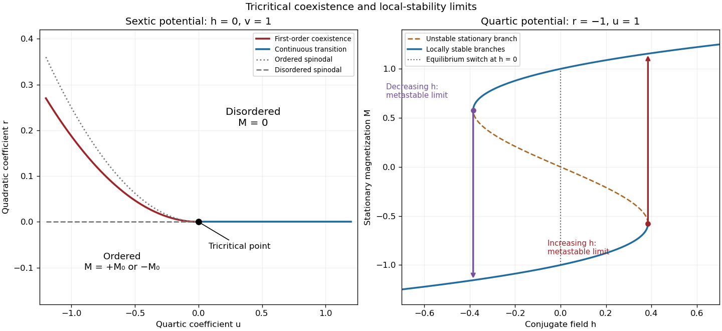
Codex 0 Created 2026-10-03 Updated 2026-10-14A tricritical point occurs when a first-order boundary meets a continuous-transition boundary. In the spin-inversion-symmetric sextic Landau free energy, two independent parameters must tune , while keeps the potential stable. In the plane, the continuous boundary is , and the first-order boundary is . They meet at the tricritical point; the order-parameter jump on the first-order side tends to zero as . The first panel shows this phase diagram, including the metastability limits derived above.
Along the tuned line , the equation of state is . Thus on a selected ordered branch, rather than the ordinary square-root behavior. Differentiation gives inverse magnetic susceptibility above and below, while at criticality . Hence the mean-field tricritical exponent calculation yields , , ; the minimized potential also gives . These tricritical powers require tuning the quartic coefficient, not merely varying a generic temperature path. The ordinary scalar exponents requested separately are calculated next.
Scalar sextic Landau phase diagram with a tricritical point, and quartic metastable hysteresis branches
. Details. Pinned article: Introduction to the OurBigBook Project
Welcome to the OurBigBook Project! Our goal is to create the perfect publishing platform for STEM subjects, and get university-level students to write the best free STEM tutorials ever.
Everyone is welcome to create an account and play with the site: ourbigbook.com/go/register. We belive that students themselves can write amazing tutorials, but teachers are welcome too. You can write about anything you want, it doesn't have to be STEM or even educational. Silly test content is very welcome and you won't be penalized in any way. Just keep it legal!
Intro to OurBigBook
. Source. We have two killer features:
- topics: topics group articles by different users with the same title, e.g. here is the topic for the "Fundamental Theorem of Calculus" ourbigbook.com/go/topic/fundamental-theorem-of-calculusArticles of different users are sorted by upvote within each article page. This feature is a bit like:
- a Wikipedia where each user can have their own version of each article
- a Q&A website like Stack Overflow, where multiple people can give their views on a given topic, and the best ones are sorted by upvote. Except you don't need to wait for someone to ask first, and any topic goes, no matter how narrow or broad
This feature makes it possible for readers to find better explanations of any topic created by other writers. And it allows writers to create an explanation in a place that readers might actually find it.
Figure 1. Screenshot of the "Derivative" topic page. View it live at: ourbigbook.com/go/topic/derivativeVideo 2. OurBigBook Web topics demo. Source. - local editing: you can store all your personal knowledge base content locally in a plaintext markup format that can be edited locally and published either:This way you can be sure that even if OurBigBook.com were to go down one day (which we have no plans to do as it is quite cheap to host!), your content will still be perfectly readable as a static site.
- to OurBigBook.com to get awesome multi-user features like topics and likes
- as HTML files to a static website, which you can host yourself for free on many external providers like GitHub Pages, and remain in full control

Figure 2. You can publish local OurBigBook lightweight markup files to either OurBigBook.com or as a static website.
Figure 3. Visual Studio Code extension installation.
Figure 5. . You can also edit articles on the Web editor without installing anything locally. Video 3. Edit locally and publish demo. Source. This shows editing OurBigBook Markup and publishing it using the Visual Studio Code extension. 
- Infinitely deep tables of contents:




All our software is open source and hosted at: github.com/ourbigbook/ourbigbook
Further documentation can be found at: docs.ourbigbook.com
Feel free to reach our to us for any help or suggestions: docs.ourbigbook.com/#contact