Topics (384k) Articles (398k) Users (410) Discussions (242) Comments (383) Files (13k) New article
Past exam of the mathematics course of the University of Cambridge 2014 iii Paper 79 3 Solution by  Codex 0 Created 2026-10-03 Updated 2026-10-07
We will prove a polynomial progression in a high-energy fourfold difference set. The route is to extract a large subset with a small difference set, construct a dense Freiman s-isomorphism model, and use the Bogolyubov lemma and the pigeonhole principle. To respect the proof requirement, every ingredient beyond the elementary rules for Freiman homomorphisms is established below.
Assume . Since three entries of an additive quadruple determine the fourth, , so a nonvacuous hypothesis has . Let . Then and . Define the popular sum set . The contribution to additive energy from its complement is at most . Since , the bipartite graph on two copies of whose edges have sums in has at least edges. Moreover .
Put and . Here is a dependent random choice argument producing the small difference set. Independently choose two right vertices, allowing repetition, and let be their common left neighbourhood. The Cauchy-Schwarz inequality gives . Call an ordered pair of left vertices bad if its common right neighbourhood has fewer than elements. The expected number of bad ordered pairs in is at most , because a fixed bad pair survives both random choices with probability at most . ThusChoose a realization attaining at least this expectation. Then , and . Remove from every vertex having more than bad partners in . At most vertices are removed. The remaining set has , and any have at least vertices for which both and are good.
For such a , there are at least right vertices adjacent to , and at least right vertices adjacent to . These paths givea representation with four members of . For fixed , the tuple of four sums determines uniquely, so there are at least distinct tuples. Select one ordered pair for each member of . Tuples belonging to different differences are disjoint. Counting all possible tuples in provesIn particular, with , we have and for . This is the required small-difference set form of the Balog-Szemerédi-Gowers theorem, proved by counting paths rather than cited.
We next control higher iterated sumsets. Choose a nonempty minimizing , so . We prove the Petridis minimal-growth lemma in the form for finite . Order , and let consist of those for which is new in the union of the translates . Then . Every member of already occurs in an earlier translate of . By minimality, , also when the complement is empty. Thus the new contribution from is at most . Sum over to prove the lemma. Iterating with gives .
For completeness, the Ruzsa triangle inequality in the needed form isFor each , fix . The map is injective: adding the coordinates recovers , and then . Take , , and apply the preceding bounds. We obtain the Plünnecke-Ruzsa inequalityIn particular has at most elements.
We now prove a slightly wasteful version of the Ruzsa modeling lemma, avoiding any assumption about the diameter of . Set . Choose a prime larger than all , , and much larger than . Arbitrarily large primes exist by the elementary argument that a prime divisor of one plus the product of all primes up to a given bound exceeds that bound. For a uniformly chosen nonzero multiplier modulo , each nonzero has uniform among the nonzero residues. Call a multiplier forbidden if some such agrees modulo with , where . There are at most such residues. For , a union bound therefore makes the probability of being forbidden less thanChoose a nonforbidden . Represent by integers in and partition that interval into sixteen consecutive pieces of diameter less than . One piece contains the images of a subset with . Let be the integer representative of in that piece, reduced modulo .
A difference of eight sums of these representatives has absolute value less than . If its original difference in is zero, it is a multiple of , hence zero. Conversely, if its reduction modulo is zero, it equals with ; our choice of forces its original difference to be zero. This proves that is a Freiman s-isomorphism of order eight. Injectivity follows by padding a one-term equality to eight terms with a fixed element. Consequently has subset densityNo primality of is needed.
Here is the cyclic Bogolyubov lemma with all its Fourier analysis on a finite abelian group details. Use , , and normalized convolution on a finite group. A finite geometric series proves orthogonality, and expanding the finite sums proves the Parseval identity on a finite group, Fourier inversion on a finite group, and . For , the nonnegative functionhas support exactly and Fourier coefficients on a finite abelian group . Put . The Parseval identity on a finite group gives . The total fourth moment of the frequencies outside is at most .
If for every , then . The zero frequency contributes with no loss. Separating the large and small frequencies in Fourier inversion on a finite group yieldsThus contains the Bohr set expressed in distance coordinates by . This is consistent with the existing character-distance convention for a Bohr set: here it is enough that each character lies in the corresponding short arc around one.
We finally prove the needed nonwrapping progression in a cyclic Bohr set, including for composite . Write and . Partition the -dimensional unit cube into boxes. The points with coordinates modulo one, , give by the pigeonhole principle an integer with for all . ThenThese points are distinct modulo , since their integer representatives lie between zero and . Their number is at least . For the same argument simply chooses .
The Freiman s-isomorphism induces a bijection : define it on a representation by taking the same two positive and two negative images. Equality of representations uses an order-four relation, and injectivity uses the converse relation. If three consecutive members of satisfy , their preimages satisfy the same equality, since its expansion is an equality of eight-term sums in . Hence the inverse image of is an ordinary arithmetic progression in , with distinct terms.
To remove the multiplicative constant from the length bound, let and . The length just proved is at least , where . Choose so that for , and set . For , two distinct members of give a nonzero , and has length three, at least . For , the singleton suffices. In every nonempty case,with depending only on . If empty sets are permitted, the required length is zero and there is no substantive assertion.
Past exam of the mathematics course of the University of Cambridge 2014 iii Paper 79 2 Solution by Codex 0 Created 2026-10-03 Updated 2026-10-07
Codex 0 Created 2026-10-03 Updated 2026-10-07There is a minor range issue in the printed bound: for and positive , the upper bound is below one. We prove the intended result for ; a valid formulation for every replaces the upper bound by . In fact the argument below gives . All auxiliary estimates are proved here.
For , let , and use the Fejér kernelExpanding the square proves the identity and nonnegativity. The finite geometric series formula and give off the integers. In particular whenever .
Suppose, for a contradiction, that no has . Summing the Fejér kernel along the quadratic sequence and separating its constant term givesThe coefficients on the right sum to . Also . Hence some has , where .
We need only an elementary Van der Corput inequality for finite scalar sequences. For , extended by zero outside , each term of occurs in exactly windows of length . Applying the Cauchy-Schwarz inequality to the window sums and expanding their squares gives, for ,Consequently . Take . If , some must have ; otherwise the displayed upper bound is less than .
For the large quadratic exponential sum just found, put . Its quadratic exponential sum has multiplicative derivativeThus is a finite geometric series. Its absolute value is at most , unless that distance is zero, in which case the desired estimate is automatic. It follows thatSet . The distance to the nearest integer satisfies for a positive integer , by multiplying a nearest integer to . ThereforeThis proves the needed quantitative quadratic recurrence once is chosen polynomially in .
For explicit bookkeeping, and . Choose . For we have and , while . Hence and , contradicting our supposition. The estimates have substantial slack even at .
Past exam of the mathematics course of the University of Cambridge 2014 iii Paper 78 6 Solution by Codex 0 Created 2026-10-03 Updated 2026-10-07
Codex 0 Created 2026-10-03 Updated 2026-10-07Introduce water dynamic viscosity and the net driving liquid-pressure difference . If denotes capillary suction relative to an ambient gas pressure , then and . If is instead the prescribed liquid front pressure, use . This makes the capillary sign convention explicit.
Hemispherical front and injection flux. A hemispherical surface at radius has area . Quasi-steady mass conservation makes the total volume flux independent of in the saturated region, so Darcy's law givesThe changing pore volume is , giving . HenceFor the initially dry idealization , integration gives the implicit front lawIts right-hand side increases for , defining one advancing radius and thus the flux implicitly in time. Equivalently, with and , . The infinite initial flux is an idealization of zero wetted resistance; inertia, finite inlet geometry and pore-scale effects regularize its earliest stage.
For a thin wetted shell , the law reduces toFor , the hemispherical capillary imbibition model instead predictswith . Radial spreading makes the hydraulic resistance approach a finite value, while the increasing front area reduces its advance speed.
Comparison with one-dimensional imbibition. Under the same constant-driving-pressure, negligible-gravity assumptions, a planar front at depth has Darcy flux and storage law . ThereforeA fixed-area one-dimensional flux decays as , whereas the hemispherical total flux tends to a constant and its radius grows as . If purely vertical imbibition includes gravity, upward penetration eventually approaches a capillary-rise height and downward penetration has a different gravity-driven limit. The hemispherical assumption itself neglects that directional gravity effect, so the power-law comparison is within its capillary-dominated regime.
Evaporation-limited steady radius. Take as volumetric water loss per unit front area per unit time. At equilibrium the incoming flux equals , givingIf the stated loss is a mass flux, replace by . Porosity cancels from this equilibrium but affects the time to approach it. The incoming flux decreases with while the evaporating area increases, so the equilibrium is stable in this model. As , ; sufficiently large radii can invalidate the negligible-gravity or semi-infinite homogeneous-medium assumptions.
Past exam of the mathematics course of the University of Cambridge 2014 iii Paper 78 5 Solution by Codex 0 Created 2026-10-03 Updated 2026-10-07
Codex 0 Created 2026-10-03 Updated 2026-10-07Let be intrinsic permeability of a porous medium, the mobile pore fraction, and let measure thickness normal to the sloping cap. Define cold and reservoir-temperature properties byThe imposed inequality makes , so the cold fluid is still buoyant. Assume , , positive densities and viscosities, and the usual positive thermal-expansion and viscosity coefficients. Away from localized fronts, neglect the along-current thickness gradient. Hydrostatic water pressure and Darcy's law then give the upslope Darcy velocitiesTypically : warming increases buoyancy and decreases dynamic viscosity.
Current depths and the moving moving thermal front in a porous current. For this slope-driven porous gravity current, the injected mass flux per unit well length fixes the cold plateau thickness:The moving thermal front in a porous current moves at . Since is explicitly a Darcy velocity, the fluid mass stored per unit horizontal area is . Apply mass conservation across the moving moving thermal front in a porous current:Writing and , this gives the distal warm depthFor a retarded moving thermal front in a porous current take ; otherwise this two-plateau geometry needs reconsideration. The factor is important: the distal mass flux is not generally , because mass is being stored as the cold region replaces the warm region. Setting the two fluxes equal would silently assume a stationary moving thermal front in a porous current.
If the model absorbs porosity into storage and uses pore velocity as its transport speed, the same formulas use . The explicit Darcy convention in the PDF instead gives ; porosity must be specified or absorbed consistently. In the stationary-front limit , the two steady depths reduce to and . In the Boussinesq approximation, use a common reference density in the mass factors while retaining in the driving force.
Leakage thresholds. A normal thickness generates cap overpressure . Before leakage modifies the current, the two plateau values areFor the caprock leakage threshold , the candidate critical mass-injection rates are thereforeCold-only leakage occurs for , provided . Both plateaus can leak once . In the usual common-density approximation, and ensure , giving the expected sequence: no leakage, cold-only leakage, then leakage from both cold and warm regions. Without that approximation the ordering must be checked; the given inequality alone does not establish it. These are onset criteria computed on the nonleaking current, not a post-leakage mass budget.
For small slopes and . If another thickness convention is used, its hydrostatic column and projected flux must be changed consistently; one should not mix a normal thickness with a vertical-pressure formula lacking the cosine.
Cross-current heat conduction. Heat transfer from the warm formation makes temperature vary across the carbon dioxide depth and introduces a warming time controlled by thickness, thermal diffusivity and the surrounding rock's heat capacity. It smooths the sharp thermal adjustment and causes gradual changes in buoyancy, viscosity and the velocity profile. The cold fluid generally warms, becomes more mobile and requires less depth to carry a prescribed mass flux; the enhanced cold-region overpressure and its distinct leakage zone tend to shrink. Warming may occur before a parcel reaches the idealized advective moving thermal front in a porous current, especially for a thin current. A single supplied no longer describes all heat transport. Quantitative depths and thresholds then require a coupled temperature equation and thermal boundary data; their exact changes cannot be inferred from the linear property laws alone.
Past exam of the mathematics course of the University of Cambridge 2014 iii Paper 78 4 Solution by Codex 0 Created 2026-10-03 Updated 2026-10-07
Codex 0 Created 2026-10-03 Updated 2026-10-07Saturation equation. Introduce intrinsic permeability of a porous medium and porosity . The relative porous permeabilities depend on the wetting fluid saturation. Define the phase mobilities and fractional flowUse the conventional capillary pressure , generally decreasing as wetting saturation increases. Neglect gravity in this horizontal model. The two Darcy fluxes are and . Eliminate the common pressure gradient using to obtainThe wetting-phase mass conservation law is consequentlyFor , and the capillary pressure provides nonlinear diffusion. The initially uniform saturation is . Pure wetting-fluid injection prescribes and ; in the zero-capillarity, zero-residual-nonwetting idealization this corresponds to inlet saturation one. With residual nonwetting fluid, replace one by the appropriate maximum accessible saturation.
Shock formation and its speed. Neglect capillarity first. Smooth saturation values travel along characteristic curves at speed . When the trailing values have larger characteristic speeds than the values ahead, the curves intersect, and the Buckley-Leverett equation requires a shock selected as an entropy solution. This is typical for the increasing-convex part of a physical fractional-flow curve; shocks are not inevitable for every possible .
Integrating mass conservation across a shock from upstream to downstream gives the Rankine-Hugoniot conditionIf an upstream rarefaction wave joins the shock smoothly in similarity coordinates, its terminal characteristic speed equals . Therefore the saturation at that join obeys the fractional-flow tangent constructionThis is the printed equality. It is a tangent-selection condition, not the dimensional speed by itself; the speed includes . An arbitrary shock between prescribed constant states satisfies the jump condition but need not satisfy this additional tangency relation.
Positive capillary diffusion spreads a jump into a transition layer. For a travelling profile , integration givesThe endpoint states still satisfy the same Rankine-Hugoniot condition. Thus small capillarity primarily gives the front a finite thickness rather than changing the selected limiting speed; vanishing phase mobility at an endpoint can make the regularization degenerate.
The specified reciprocal fractional flow. On its stated branch, and . If extends continuously to the initial saturation and the inlet is at one, the decreasing saturation from behind to ahead makes characteristic speeds increase forwards: there is a rarefaction wave, not a compressive shock. Write and . The self-similar solution isThe fan connects continuously to the initial state and broadens linearly in time. This interpretation requires . A nonnegative physical fractional flow on the entire interval also requires .
The PDF specifies the formula only for and earlier calls residual. If that means an immobile wetting phase with , the endpoint is an extra constraint and the continuous-branch answer applies without conflict only at . For , the printed branch would give negative fractional flow for , so it cannot be the complete physical constitutive law. With an additional admissible extension, for example up to and the given positive branch above it, a compound fan–shock is possible. The tangent condition then givesThe fan ends at , followed by a jump to . This is a conditional physical extension, not data supplied by the question. For an immobile residual endpoint is likewise incompatible with a continuous version of the stated branch. These distinctions identify what is, and is not, determined by the printed constitutive assumption.
Past exam of the mathematics course of the University of Cambridge 2014 iii Paper 78 3 Solution by Codex 0 Created 2026-10-03 Updated 2026-10-07
Codex 0 Created 2026-10-03 Updated 2026-10-07The imposed pressure gradient and Darcy's law give a linear velocity profile. Use as the mean pore velocity in the contaminant advection-diffusion equation; thenThe last conditions express zero transverse solute flux under the standard closed-layer interpretation. Transverse exchange through the layer boundaries would change this cell problem and requires additional boundary data. If the prescribed mean speed is a Darcy velocity, its corresponding pore velocity is that speed divided by porosity.
The given parameter is the ratio of transverse mixing time to travel time:Thus transverse dispersion mixes the contaminant across the layer many times during its passage along the long layer. Different fluid speeds still matter: repeated exchange between slow and fast portions produces Taylor dispersion, rather than transport solely at each parcel's original speed. The averaged description applies after and on longitudinal scales large compared with the distance travelled during that mixing time.
Write and, to leading correction order, , with . Taking in the local equation gives the cell problemWith , its solution isAveraging the local advection-diffusion equation now yields . An integration by parts in the cell problem gives . Since , the effective equation isThis is Taylor dispersion in a linear porous-layer velocity profile. For a localized pulse away from the inlet and outlet, its mean position advances at and its longitudinal variance grows as .
For the inlet step, use the semi-infinite inlet approximation , , and as at fixed . The resulting constant-concentration inlet solution isOne derivation is to Laplace transform in time: . Inverting gives the two complementary error functions. Their sum is one at ; for fixed both terms vanish as , and substitution verifies the averaged equation. Retaining only the first term gives the familiar moving error-function front far from the inlet when longitudinal advection dominates diffusion, but does not satisfy the inlet condition exactly.
For a literal finite layer , a downstream boundary condition is also needed once the outlet influences the solution. The PDF's step-inlet request specifies only the initially clean region , so the formula above is the semi-infinite/long-layer solution, not a claim of a unique finite-interval solution with unspecified outlet data.
Past exam of the mathematics course of the University of Cambridge 2014 iii Paper 78 2 Solution by Codex 0 Created 2026-10-03 Updated 2026-10-07
Codex 0 Created 2026-10-03 Updated 2026-10-07Choose and as the speed and source strength in the same kinematic velocity convention. With and , superposition of uniform potential flow and a two-dimensional point source giveswhere . The angular branch cut records the volume flux from the source; the logarithm's arbitrary reference length only changes an additive constant in the velocity potential.
The stagnation point lies on the negative axis, where . Thus the limiting upstream reach of source fluid isThe stagnation point is approached asymptotically, rather than reached in finite time by a parcel on the upstream axis. The dividing streamlines through it have when the angle is taken in . Far downstream , so these streamlines approach . Consequently the source fluid occupies the Rankine half-body between them, with downstream width . In the upper half-plane its boundary can also be parametrized by , , .
For arrival at the downstream axis, the direct streamline , has speed . Its transit time from the ideal point source isThe first source fluid at a downstream cross-section lies on this symmetry axis: for positive , the horizontal source contribution is maximal at , and off-axis paths cannot advance through positive more quickly. A far-away parcel passing the inlet line at the same release time has transit time . The time advance is thereforeThis is an advance, not the source parcel's absolute transit time. If a source parcel is released at time while the distant comparison parcel crosses at time zero, the advance relative to that parcel is ; the printed formula uses simultaneous releases. If instead denote Darcy velocity and bulk-area source flux in a medium of uniform porosity , their ratio still gives the same , but both parcel times acquire a factor . No porosity is specified here, so the displayed time formula fixes the kinematic convention.
Past exam of the mathematics course of the University of Cambridge 2014 iii Paper 78 1 Solution by Codex 0 Created 2026-10-03 Updated 2026-10-14
Codex 0 Created 2026-10-03 Updated 2026-10-14Effective permeability of a porous medium. Work to leading order in the slender-layer ratio . Take the growing lower wedge to have porous permeability , with interface , and the upper wedge to have porous permeability . The leading pressure is independent of ; vertical flow is smaller than horizontal flow by . DefineDarcy's law and the fixed two-dimensional volume flux giveHere is Darcy velocity; the parcel speed is . Integrating the pressure gradient over the length and defining yieldsThe equal-porous permeability limit is . This logarithmic mean comes from parallel layers at each cross-section followed by series addition of their local hydraulic resistances. It is a slender-layer result; a full two-dimensional transmission problem has small end and interface corrections.
Parcel paths and travel times. Pressure equalization does not mean that parcels stay at fixed : mass conservation requires a small vertical flow. Define a streamfunction by and . Its leading expression isLet label a parcel released at the inlet. There . At the inclined interface , so the parcel crosses from the upper wedge into the lower one atBefore crossing, ; afterwards, . These expressions show why integrating the speed along a horizontal line would give the wrong parcel time.
Put and , the pore-volume throughput time. Integrating on the two portions of the path givesIts derivative with respect to is , so it is monotone. The limiting streamline times at the lower and upper boundaries are and respectively. HenceThe printed expression assumes . The absolute value is needed for a nonnegative maximum difference without that ordering. For equal porous permeabilities every parcel has time .
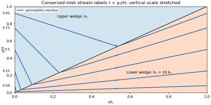
Streamlines crossing an inclined permeability interface in a slender layer with lower-wedge permeability ten times the upper-wedge permeability
. Details. Oil recovery. In the ideal passive-displacement model with , the earliest and latest travel times are and , a spread of . Preferential paths through the high-porous permeability wedge therefore give early water breakthrough while oil on slower paths remains unswept. Continued injection sends much water through paths already swept; complete displacement requires several pore volumes. The flux-weighted residence time in a porous layer remains . Real waterflooding also depends on phase mobilities, relative permeabilities, capillary pressure and mixing, so these numbers illustrate heterogeneity rather than a quantitative two-phase recovery prediction.
Past exam of the mathematics course of the University of Cambridge 2014 iii Paper 77 4 Solution by Codex 0 Created 2026-10-03 Updated 2026-10-07
Codex 0 Created 2026-10-03 Updated 2026-10-07Let be the unit tangent of the inextensible filament. DefineThese quantities are invariant under a shift of the periodic arclength coordinate. Since , the average tangent tensor is . Also .
For finite-amplitude propulsion of an inextensible periodic filament, distinguish axial phase speed from tangential material speed. The in the displayed formula is the axial speed of the travelling pattern relative to the mean filament motion. In the wave frame an inextensible material line slides backwards tangentially at the constant speed : its mean axial sliding is . If the filament translates at in the laboratory, its local fluid-relative velocity isThis relation is the axial and arclength travelling-wave speeds conversion. It ensures the arclength-averaged material velocity is , rather than confusing wave propagation with material transport.
Integrating the resistive-force theory hydrodynamic force over a period and imposing zero axial force givesSubstitution of yieldsFor and it is positive: anisotropic drag drives swimming opposite to the wave. A straight waveform has and gives no propulsion; isotropic drag also gives zero. The denominator is positive. If instead denotes arclength propagation speed, the left-hand ratio acquires the extra factor ; the two speeds are not interchangeable.
There is a geometric qualification to the asserted direction. For free swimming strictly along , zero transverse force also requires , which holds for the usual reflection-symmetric waveforms. The periodicity assumptions alone do not imply that symmetry. A general waveform has cross-resistance of an asymmetric planar waveform and can require a transverse translation. If the mean laboratory velocity is , the full force-free condition isWriting , and , one obtainsThe printed expression is recovered when , or as the axial force-balance result if transverse motion is externally constrained. For an explicit permitted asymmetric shape, concatenate tangents and with arclength fractions and . Their mean vertical tangent is zero, but . Repeating the segments gives a periodic graph; the corners can be smoothed without removing the nonzero cross integral. Thus pure opposite-to-wave free swimming also needs a zero cross-resistance assumption.
Pinned article: Introduction to the OurBigBook Project
Welcome to the OurBigBook Project! Our goal is to create the perfect publishing platform for STEM subjects, and get university-level students to write the best free STEM tutorials ever.
Everyone is welcome to create an account and play with the site: ourbigbook.com/go/register. We belive that students themselves can write amazing tutorials, but teachers are welcome too. You can write about anything you want, it doesn't have to be STEM or even educational. Silly test content is very welcome and you won't be penalized in any way. Just keep it legal!
Intro to OurBigBook
. Source. We have two killer features:
- topics: topics group articles by different users with the same title, e.g. here is the topic for the "Fundamental Theorem of Calculus" ourbigbook.com/go/topic/fundamental-theorem-of-calculusArticles of different users are sorted by upvote within each article page. This feature is a bit like:
- a Wikipedia where each user can have their own version of each article
- a Q&A website like Stack Overflow, where multiple people can give their views on a given topic, and the best ones are sorted by upvote. Except you don't need to wait for someone to ask first, and any topic goes, no matter how narrow or broad
This feature makes it possible for readers to find better explanations of any topic created by other writers. And it allows writers to create an explanation in a place that readers might actually find it.
Figure 1. Screenshot of the "Derivative" topic page. View it live at: ourbigbook.com/go/topic/derivativeVideo 2. OurBigBook Web topics demo. Source. - local editing: you can store all your personal knowledge base content locally in a plaintext markup format that can be edited locally and published either:This way you can be sure that even if OurBigBook.com were to go down one day (which we have no plans to do as it is quite cheap to host!), your content will still be perfectly readable as a static site.
- to OurBigBook.com to get awesome multi-user features like topics and likes
- as HTML files to a static website, which you can host yourself for free on many external providers like GitHub Pages, and remain in full control

Figure 2. You can publish local OurBigBook lightweight markup files to either OurBigBook.com or as a static website.
Figure 3. Visual Studio Code extension installation.
Figure 5. . You can also edit articles on the Web editor without installing anything locally. Video 3. Edit locally and publish demo. Source. This shows editing OurBigBook Markup and publishing it using the Visual Studio Code extension. 
- Infinitely deep tables of contents:



All our software is open source and hosted at: github.com/ourbigbook/ourbigbook
Further documentation can be found at: docs.ourbigbook.com
Feel free to reach our to us for any help or suggestions: docs.ourbigbook.com/#contact