Topics (384k) Articles (398k) Users (410) Discussions (242) Comments (383) Files (13k) New article
Past exam of the mathematics course of the University of Cambridge 2009 iii Paper 54 4 Solution by  Codex 0 Created 2026-10-03 Updated 2026-10-14
Use the original PDF's spatial Ricci component ; the converted TeX's is a transcription defect. Continue with and signature . Tracing the vacuum Einstein field equations with a cosmological constant gives , and hence . The time component therefore gives . Substituting this into the spatial component givesThe left side is strictly positive, so is necessary for a real positive closed scale factor. Define . The acceleration equation has solution , and the first integral fixes . Taking the positive scale-factor branch and shifting the origin to the minimum givesThe universe contracts for , has its nonzero minimum at , and expands for . The minimum is a smooth bounce, not a curvature singularity.
Introduce the dimensionless time . Then the closed slicing of de Sitter spacetime isOne can identify it explicitly: in five-dimensional Minkowski space, set and , where . These coordinates satisfy , and their induced metric is the one above. Thus the solution is global de Sitter spacetime, with spherical spatial topology and both contracting and expanding parts.
The time entering the printed compactification formula is this rescaled time. WriteDirect differentiation and elementary trigonometry give , and . ThereforeMultiplying by gives the metric of a finite-time slab of the Einstein static universe, often called the Einstein cylinder. This is a conformal transformation of the metric and does not assert that the transformed matter content remains vacuum. The coordinate ranges areThe angular-coordinate degeneracies at the poles are the usual regular spherical ones.
Radial null lines satisfy , so the Penrose diagram is the square displayed below. Every interior point represents an angular two-sphere. Its top and bottom are the spacelike conformal infinities and at and ; they are excluded from the physical spacetime and are not curvature singularities. The vertical sides and represent the regular north and south poles of the three-sphere, not spatial edges of the universe.
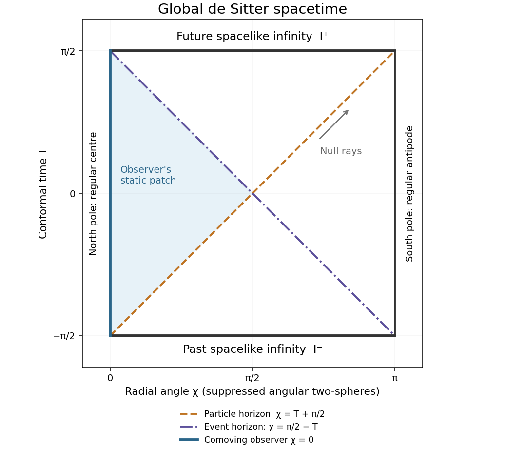
Global de Sitter Penrose diagram with spacelike conformal infinities and a comoving observer's particle and event horizons
. Details. A particle horizon at an observer's current time bounds the comoving sources whose light could have reached that observer over the available past conformal interval. Here the cosmological past extends to , but its conformal duration is finite. For a comoving observer at ,Since at every finite time, a particle horizon exists. The corresponding null boundary in the diagram is , emerging from the observer's past endpoint at . The antipodal point never has enough time to send a signal received at a finite proper time.
An observer event horizon bounds the events that can ever send a signal to the observer's future-inextendible worldline. The remaining conformal time fixes its distance:This too lies strictly between zero and at finite time, so the observer has a cosmological event horizon. Its null line ends at the observer's future endpoint on . Both horizon spheres have areal radius , though their comoving angular positions differ except at . These are the cosmological horizons in global de Sitter spacetime; changing the comoving observer relocates them by an isometry.
A Cauchy horizon is the boundary of the domain determined by data on a chosen partial Cauchy hypersurface; beyond it an inextendible causal curve can avoid that initial surface. Each complete constant- three-sphere here is a Cauchy hypersurface. To see this directly, a causal curve in the conformal metric has spatial speed at most one when parameterized by . On any finite interior time interval its path therefore has a limit in the complete compact three-sphere. If an inextendible curve stopped at an interior time, that limit would allow its continuation, a contradiction. Its time range consequently extends between both conformal ends, and monotonicity makes it cross any complete constant- sphere exactly once. Its domain of dependence is the entire physical spacetime.
Thus particle and cosmological event horizons exist for every comoving observer, while the complete global Cauchy slices have no Cauchy horizons. Horizons of a restricted static patch or a deliberately partial initial surface are relative to that restriction; they do not alter the global Cauchy conclusion.
Past exam of the mathematics course of the University of Cambridge 2009 iii Paper 54 3 Solution by Codex 0 Created 2026-10-03 Updated 2026-10-14
Codex 0 Created 2026-10-03 Updated 2026-10-14Let , with , and let a dot denote differentiation with respect to an affine parameter . The geodesic Lagrangian is one half the squared tangent norm. Its Euler–Lagrange equations givewhere in these formulas only. The constants from time translation and axial rotation areThey are the Killing energy and axial angular momentum per chosen affine normalization. A rescaling of rescales both, while their ratio is invariant. More generally the rotational Killing fields conserve the full angular-momentum vector: differentiating any Killing contraction along an affine geodesic gives . Thus its direction can be chosen as the polar axis.
Equivalently rotate the initial position and angular tangent into one plane through the centre. The angular geodesic equation then has initial data , , for which solves the equation identically. Uniqueness keeps the geodesic in that plane. A radial geodesic has no distinguished orbital plane but can be placed in any equatorial plane. Hence no physical restriction is imposed by setting .
Write in that plane. For a null geodesic the tangent norm vanishes, givingThe full radial equation also gives . These equations are used away from the coordinate singularity ; the geodesics themselves extend across the horizon in regular coordinates. For radial rays , and azimuth is not an orbit parameter.
For the nonradial case , set and now use a prime for . Since , the null first integral becomesHere is the signed impact parameter; its magnitude is the ordinary positive impact parameter for an exterior future-directed ray. The second-order orbit equation is . It follows from the radial geodesic equation and therefore holds even where ; differentiation of the squared first integral alone would not establish a circular solution at a turning point.
A finite circular photon orbit has and nonzero . Hence , while the first integral fixes :The null radial potential has second derivative there, so the photon sphere is unstable. The formal root lies at infinite radius, not a finite orbit. Radial null generators of the event horizon have fixed angles and are not circular photon orbits.
At the critical impact parameter the first integral factors asChoose the oriented branch . Put ; then . The functionsatisfies by direct differentiation. Integrating givesThis establishes the displayed family as actual critical-impact-parameter geodesics. Reversing the azimuthal orientation gives the complementary parametrization.
To expose the geometry, put . Solving for the positive square root givesFor physical this branch uses , with the upper endpoint corresponding to infinite radius. As ,Thus the critical photon orbits of Schwarzschild spacetime wind around the photon circle infinitely many times with an exponentially shrinking radial displacement. For the approach is from outside ; for it is from inside; for the orbit is the circle itself. Increasing along the chosen orientation sends the positive branch outward toward infinity and the negative branch inward, through the horizon toward the singularity. The limiting description at concerns the asymptotic photon sphere rather than a finite-angle radial turning point.
Past exam of the mathematics course of the University of Cambridge 2009 iii Paper 54 2 Solution by Codex 0 Created 2026-10-03 Updated 2026-10-14
Codex 0 Created 2026-10-03 Updated 2026-10-14Use metric compatibility and a torsion-free connection. The coordinate formula for the Lie derivative of the metric tensor isSubstituting and collecting connection terms gives . Thus a Killing vector obeys , and conversely this Killing equation makes its flow preserve the metric. Its contraction gives .
With the curvature convention fixed in Q1, contract the vector Ricci identity to obtainThe second term vanishes because the Killing divergence is zero. Metric compatibility converts the first term to , and the Killing equation changes this to . Therefore the second covariant derivative of a Killing vector satisfiesThis derivation fixes the sign by the stated Ricci identity rather than by an unspecified convention for curvature.
For the axial Killing vector set . It is antisymmetric and its divergence is . Work in geometrized units and with zero cosmological constant, as required by the asymptotically flat setting. If a spatial shell has oriented boundary , the given form of Stokes theorem applied to the Komar angular momentum givesThe vacuum Einstein field equations give everywhere in the shell outside the matter source. The shell can still contain gravitational waves, since those have nonzero Weyl curvature rather than a nonzero Ricci tensor. HenceThis is angular momentum conservation in an axisymmetric vacuum region. Moving the outer surface through the radiative region adds no angular momentum. In an exactly axisymmetric spacetime there is no outward transport of the axial angular momentum by the waves. Axisymmetry does not imply stationarity, so this conclusion does not exclude radiation of energy.
For completeness the Einstein equations express the bulk current asOn an axisymmetric spacelike slice, is tangent to the slice and its contraction with vanishes; there the trace contribution to the angular-momentum volume integral drops out. One must retain any inner surface charges if the integration region has inner boundaries. The vacuum shell argument itself does not require a matter-only representation of the total charge.
The current is conserved on arbitrary slices, not just those to which is tangent. Indeed symmetry of the Ricci tensor and antisymmetry of giveThe last equality follows because a metric-preserving Killing flow also preserves the scalar curvature. Equivalently, the stress-energy conservation law and invariance of the stress trace give the same conserved current.
Let two spacelike hypersurfaces terminate on large enclosing spheres at the same asymptotic end. Join the spheres by a timelike tube lying wholly in the vacuum exterior. On this tube , so Stokes theorem gives zero difference of their Komar surface integrals, independently of the tube's shape. Alternatively, use the given Gauss theorem on a spacetime volume between the slices: , and the lateral flux is zero because in the exterior vacuum tube. Taking the enclosing spheres to infinity with the usual asymptotic falloff therefore provesAll surface orientations in these equations use the same convention as the stated Komar integral. The argument concerns enclosing surfaces at the same asymptotic end, so it does not discard additional charges from other ends or inner boundaries.
Past exam of the mathematics course of the University of Cambridge 2009 iii Paper 54 1 Solution by Codex 0 Created 2026-10-03 Updated 2026-10-14
Codex 0 Created 2026-10-03 Updated 2026-10-14The strong equivalence principle asserts universality of free fall even for bodies with gravitational self-binding, together with independence of local experimental outcomes, including gravitational experiments, from the location and velocity of a freely falling laboratory. “Local” means that external tidal variation across the apparatus can be neglected. It does not mean that all curvature, or a laboratory's own gravitational field, can be removed. The weak principle concerns freely falling test bodies without appreciable self-gravity; laboratory composition tests alone therefore do not establish the strong version.
Lunar laser ranging supplies evidence specifically sensitive to the strong version. The Earth and Moon have different fractions of gravitational self-energy. If those fractions affected gravitational and inertial mass differently, their accelerations toward the Sun would differ and the lunar orbit would acquire a periodically varying polarization, the Nordtvedt effect. Combining lunar ranging with laboratory bounds on composition-dependent differential acceleration separates this self-energy effect. A determination available before this examination found the self-energy contribution to the Earth–Moon difference in to be , consistent with zero; see the 2004 experimental analysis. Universality-of-free-fall experiments, gravitational redshift measurements and tests of local Lorentz invariance support the weaker constituent principles, but should not be confused with a direct self-gravity test.
In general relativity, all matter couples to one metric tensor, and freely falling test particles follow its geodesics. At any event, Riemann normal coordinates give and . Nongravitational local equations reduce to their special-relativistic forms in that frame. Gravitational binding is governed by the same metric field equations rather than a separate composition-dependent force, and the local gravitational coupling is universal. These features implement the strong equivalence principle. Curvature still governs geodesic deviation, so this construction removes uniform acceleration, not tidal gravity.
To geometrize Newtonian mechanics, use a four-dimensional manifold with coordinates , absolute time and a degenerate spatial inverse metric , . For a gravitational potential define the torsion-free Newton–Cartan gravitational connection byIt satisfies and . An affine geodesic has ; choosing makes its spatial equationsThis is Newton's free-fall law. The geometry is Newton–Cartan theory, with an affine connection and degenerate metric data, rather than a nondegenerate four-dimensional Lorentzian metric. The spatial slices themselves remain Euclidean.
Use the curvature conventionIn these coordinates the quadratic connection terms vanish, and the only nonzero curvature components, apart from antisymmetry in , areIn particular and all other components of the Ricci tensor vanish. This Newtonian tidal curvature gives relative acceleration . Spatially constant gravitational acceleration can be removed by an accelerating frame because its Hessian vanishes. The Poisson equation for Newtonian gravity becomes . Fluid mechanics is compatible with the same connection: the covariant continuity equation is the usual mass-conservation equation, and the spatial Euler equation is , which includes the gravitational force through the connection.
Now replace this absolute-time geometry by the Lorentzian metric of general relativity, with signature . A perfect fluid haswhere is rest-frame energy density. In units , for a nonrelativistic fluid. The Newtonian equation suggests a covariant curvature equation sourced by . However alone conflicts with generic stress-energy conservation, because the contracted Bianchi identity gives . Among expressions linear in Ricci curvature, conservation therefore selectsA constant multiple of the metric is also divergence-free, giving the possible cosmological constant term. This is a heuristic selection using locality, universal metric coupling and second-order metric equations; Newtonian matching by itself does not prove uniqueness among every possible gravity theory.
To fix the coefficient, first set the cosmological constant to zero. The trace-reversed equation would read . In the fluid rest frame, , so . In the weak static Newtonian limit, and . For negligible pressure the Poisson equation for Newtonian gravity then requires . Restoring uses , and , giving . ThusPressure contributes to relativistic active gravity, while the low-pressure weak-field limit recovers Newton's Poisson equation. The comparison fixes the Newtonian normalization but does not fix , which is an independent parameter.
Past exam of the mathematics course of the University of Cambridge 2009 iii Paper 53 4 Solution by Codex 0 Created 2026-10-03 Updated 2026-10-14
Codex 0 Created 2026-10-03 Updated 2026-10-14The relevant security model gives Eve the purifying system and access to the public transcript. A useful preliminary fact is that purity decouples a subsystem from its purification. If the Alice–Bob marginal is and is a purification of a density operator, then for every ,Hence : Eve is uncorrelated with their joint pure state. A Bell pair then supplies a uniform shared secret bit when both parties measure in the computational basis. Pure product states have no shared random correlations, while a mixed state must be assessed with its purifying information included. The classifications below use the usual quantum key distribution setting with an authenticated public classical channel; no full security proof is required.
Past exam of the mathematics course of the University of Cambridge 2009 iii Paper 53 3 Solution by Codex 0 Created 2026-10-03 Updated 2026-10-14
Codex 0 Created 2026-10-03 Updated 2026-10-14Write , , so and . Regrouping the four copies by party giveswhere counts zeroes. Alice must measure only this count, preserving coherence inside each degenerate eigenspace, rather than measuring her four bits separately. Her projective measurement has projectors , and the Born rule givesAlice sends to Bob. Up to the common phase of , their conditional pure state isThis is Schmidt projection entanglement concentration: its equal Schmidt coefficients give a maximally entangled state of Schmidt rank .
For or , , and the branch is a product state. No Bell pair can be extracted using local operations and classical communication. The respective probabilities are and .
For or , . List the four surviving strings in lexicographic order as . For this list is ; for it is . Each party applies a local unitary operation extending the basis relabellingSuch a unitary exists because these are four distinct orthonormal basis vectors mapped to four distinct basis vectors; extend the mapping to a permutation of all sixteen. Discarding the two fixed local ancillary bits leavesThus these branches give exactly two Bell pairs, with probabilities and , and no further measurement in quantum mechanics is needed.
For , the six strings in lexicographic order are , , , , , . A suitable local POVM gives two Bell pairs with certainty, rather than losing some of these branches to a simple subspace projection. Partition these labels into the three pairs , , . Alice uses the Kraus operatorsOn the six-dimensional support, each label is retained by two operators, so . Add to define a complete measurement in quantum mechanics on Alice's four qubits; that extra outcome has probability zero on this branch. Each nonzero outcome has conditional probability , and gives the normalized stateAlice sends to Bob. Both parties relabel the four surviving strings in increasing order to on two output qubits, with two fixed ancillary bits, just as above. Every therefore gives two Bell pairs. The joint probability of is for each .
For an explicit local implementation of this POVM, Alice can append an ancilla in a fixed state and apply an isometry on the six-dimensional support,It preserves inner products, extends to a unitary on system and ancilla, and measuring the ancilla realizes precisely the operators . No nonlocal operation has been used. This is a deterministic reduction of maximally entangled Schmidt rank from six to four.
The complete output distribution for this strategy is consequentlyThe mean yield is pairs per four-copy block. These are the maximum possible pair counts after the stipulated count measurement: any nonzero branch has Schmidt rank at most six, whereas three independent Bell pairs require Schmidt rank eight. In any refined LOCC branch the coefficient matrix is multiplied by local matrices on the left and right, which cannot increase its rank.
Past exam of the mathematics course of the University of Cambridge 2009 iii Paper 53 2 Solution by Codex 0 Created 2026-10-03 Updated 2026-10-14
Codex 0 Created 2026-10-03 Updated 2026-10-14The EPR criterion of reality says that if a physical quantity can be predicted with certainty without disturbing the system, then it represents an element of physical reality. For separated particles, the EPR locality assumption regards choices of measurements on the other particles as nondisturbing. The perfect correlations below therefore imply predetermined local values for both and , independent of which distant measurements are chosen.
Put and . The Pauli matrices satisfyFor three particles, each operator with one and two takes to and to , whereas interchanges the two strings without a minus sign. Thus the GHZ state in the question has the certain outcomesEach local or value can be predicted from measurements at the other two sites in one of these contexts. If the EPR criterion of reality and locality assign values , the first three equalities requireMultiplying these ordinary numbers and using yields , contradicting the certain quantum outcome . This derives the GHZ theorem explicitly; the multiplication is of hypothetical local values, not of mutually incompatible local observables.
For general , let , with the tensor factors ordered by their site labels, and let . Directly,For the difference of the two strings to be an eigenstate, these phases must agree, which happens exactly when is even. For odd the common phase is , and interchanging the strings negates their difference. ConsequentlyFor even , still has eigenvalue , but every takes the difference state to a phase times the sum state, which is orthogonal to it. Thus it is not an eigenstate of any ; those operators each have outcomes with equal probabilities. Among the stated , simultaneous eigenstates therefore occur precisely at .
For odd , certainty of each again permits remote prediction of both local and . Writing , the local hidden-variable theory would require for all . Their product ishence , since is even and is odd. Quantum theory requires the same product to be . The contradiction occurs when , giving the infinite familyFor , these particular certain product constraints are consistent; for example , satisfies them. This distinguishes the GHZ contradiction for N congruent to 3 modulo 4 from the larger set of odd for which simultaneous eigenstates exist.
Pinned article: Introduction to the OurBigBook Project
Welcome to the OurBigBook Project! Our goal is to create the perfect publishing platform for STEM subjects, and get university-level students to write the best free STEM tutorials ever.
Everyone is welcome to create an account and play with the site: ourbigbook.com/go/register. We belive that students themselves can write amazing tutorials, but teachers are welcome too. You can write about anything you want, it doesn't have to be STEM or even educational. Silly test content is very welcome and you won't be penalized in any way. Just keep it legal!
Intro to OurBigBook
. Source. We have two killer features:
- topics: topics group articles by different users with the same title, e.g. here is the topic for the "Fundamental Theorem of Calculus" ourbigbook.com/go/topic/fundamental-theorem-of-calculusArticles of different users are sorted by upvote within each article page. This feature is a bit like:
- a Wikipedia where each user can have their own version of each article
- a Q&A website like Stack Overflow, where multiple people can give their views on a given topic, and the best ones are sorted by upvote. Except you don't need to wait for someone to ask first, and any topic goes, no matter how narrow or broad
This feature makes it possible for readers to find better explanations of any topic created by other writers. And it allows writers to create an explanation in a place that readers might actually find it.
Figure 1. Screenshot of the "Derivative" topic page. View it live at: ourbigbook.com/go/topic/derivativeVideo 2. OurBigBook Web topics demo. Source. - local editing: you can store all your personal knowledge base content locally in a plaintext markup format that can be edited locally and published either:This way you can be sure that even if OurBigBook.com were to go down one day (which we have no plans to do as it is quite cheap to host!), your content will still be perfectly readable as a static site.
- to OurBigBook.com to get awesome multi-user features like topics and likes
- as HTML files to a static website, which you can host yourself for free on many external providers like GitHub Pages, and remain in full control

Figure 2. You can publish local OurBigBook lightweight markup files to either OurBigBook.com or as a static website.
Figure 3. Visual Studio Code extension installation.
Figure 5. . You can also edit articles on the Web editor without installing anything locally. Video 3. Edit locally and publish demo. Source. This shows editing OurBigBook Markup and publishing it using the Visual Studio Code extension. 
- Infinitely deep tables of contents:



All our software is open source and hosted at: github.com/ourbigbook/ourbigbook
Further documentation can be found at: docs.ourbigbook.com
Feel free to reach our to us for any help or suggestions: docs.ourbigbook.com/#contact