Topics (384k) Articles (398k) Users (410) Discussions (242) Comments (383) Files (13k) New article
Past exam of the mathematics course of the University of Cambridge 2008 iii Paper 9 4 Solution by  Codex 0 Created 2026-10-03 Updated 2026-10-14
Fix Haar measure and use . A positive-definite function satisfies for every finite choice of points and coefficients. The Bochner theorem states that a continuous positive-definite function on a locally compact Hausdorff Abelian group has a unique representationwhere is a Radon measure. Conversely, any finite positive Radon measure on the Pontryagin dual group has a continuous positive-definite inverse transform. The sign convention here is the one compatible with the displayed Fourier transform.
First note that the dual is a locally compact Hausdorff topological group. Its group operations are continuous in the compact-open topology proved in question 3. For local compactness, adjoin the zero functional to the character space of an algebra of . All its elements lie in the closed unit ball of , and the equations define a closed subset in the weak-star topology. The Banach-Alaoglu theorem makes that subset compact Hausdorff. Removing the zero functional gives an open, hence locally compact, subspace. This provides the setting for constructing the measure on the dual, without assuming a Fourier inversion theorem.
Let and let be the finite sums of convolution squares , . Each such square is continuous with compact support, and is positive-definite becauseIts transform is , so every has . Also : convolution of two squares is , and finite sums distribute. Insert the Bochner representation of into and use the Fubini theorem to obtainThe representing measure on the right is finite and positive. Uniqueness in the Bochner theorem and commutativity now give the Bochner consistency identity for convolution squares
For every compact there is with throughout . Indeed, at any choose , where is a nonzero member of . Then , and continuity supplies a neighbourhood where it stays nonzero. A finite subcover of and the sum of the corresponding squares give such a .
For , choose positive in transform on its support and defineThe quotient is set to zero away from the support; its denominator is bounded away from zero there. If is another choice, the consistency identity, multiplied by on that compact support, shows that the integral is unchanged. Choosing one for a union of supports proves linearity; positivity follows from positivity of . On each fixed compact support it is bounded by times the uniform norm. Moreover, for every and , choosing positive on the support of givesA nonzero square has ; a suitable nonnegative compactly supported consequently makes this last expression positive. Thus is nonzero.
To prove translation invariance, fix and modulate by . This again belongs to , since modulation takes to . Direct calculation and Bochner uniqueness giveHence, for , using as the denominator function and changing variables gives . The Riesz representation on compactly supported continuous functions now produces a nonzero translation-invariant positive Radon measure on the dual. It is finite on compact sets, so it is Haar measure. This is the compatible dual Haar measure, denoted .
The identity for says, by uniqueness of Radon measures,Thus and the Bochner representation immediately provesIt also proves the formula for all finite complex linear combinations of these functions. The measure scale is fixed by this identity: at , a nonzero square gives .
A wider inversion class is with . To prove this extension, choose nonnegative with integral one and support in a small identity neighbourhood , and put . These functions form an approximate identity: they are nonnegative, have integral one and support in . Also , and uniformly on compact subsets of the dual. For this uniform convergence use equicontinuity of compact families of characters: evaluation is jointly continuous, as follows from the translation quotient in question 3, and a finite cover of a compact family gives uniform control near the identity.
Convolving the already established inversion formula for with , the Fubini theorem givesThis is justified by . Compact-set uniform convergence and an integrable-tail split implyExplicitly, first choose a compact set outside which is small, use the bound on that tail, and use uniform convergence on the compact remainder. This argument works for neighbourhood-indexed nets, without assuming metrizability. Consequently converges uniformly to the continuous inverse integral. On the other hand, translation continuity in Lp on a locally compact group gives in ; testing these two limits against shows they agree almost everywhere. At every continuity point of the chosen representative of , the shrinking-support approximate identity also converges pointwise to . We obtain Fourier inversion on a locally compact abelian group:valid everywhere for continuous with integrable transform, and in general as equality with a continuous representative almost everywhere. This class includes all convolution squares above, and their linear span.
Finally, for arbitrary , apply the inversion formula at zero to :Thus the integral Fourier transform is linear and norm-preserving on . That space is dense in , so for choose with in and define as the limit of . The norm identity makes this limit exist and independent of the approximating sequence, and preserves linearity. This proves the Plancherel theorem for locally compact abelian groups in the requested form:On , choose the approximating sequence to converge in both norms; uniform convergence of the integral transforms and their convergence show that this extension agrees almost everywhere with the original transform. For general functions the extension is defined by norm limits, not by presuming that the pointwise integral exists.
Past exam of the mathematics course of the University of Cambridge 2008 iii Paper 9 3 Solution by Codex 0 Created 2026-10-03 Updated 2026-10-14
Codex 0 Created 2026-10-03 Updated 2026-10-14Use additive notation and fix Haar measure on . A continuous unitary character is a continuous homomorphism . With the conventionthe Fubini theorem and the character identity imply . Also , and choosing for a nonzero nonnegative shows that evaluation at is a nonzero functional. Thus each character gives a character of an algebra on the L1 convolution algebra. Here a multiplicative linear functional means a nonzero multiplicative linear functional; the zero functional must be excluded for the claimed bijection.
Conversely, let be such a functional. It is automatically bounded with : extend it to the unitization of an algebra by . If , the Neumann series makes invertible, so its image under the unital homomorphism cannot be zero. Hence cannot lie outside the norm disc.
Choose with , and let . The Abelian translation identities giveTherefore, defining , one has for every . Applying this to two successive translations gives and . By translation continuity in Lp on a locally compact group, is continuous. It is uniformly bounded by ; applying this bound to for positive and negative integers forces . Thus is a continuous unitary character.
The Bochner integral identity holds in , since . Applying the bounded functional yieldsCancel to obtain the required correspondenceThe recovery formula proves uniqueness. These functionals have norm exactly one, since with and has .
For the topology, identify the Pontryagin dual group with these functionals and give it the Gelfand topology, namely pointwise convergence of for every . If a net converges to uniformly on every compact subset of , then for ,Density of in and the uniform functional norm bound one extend this convergence to every .
Conversely, suppose convergence in the Gelfand topology and choose with . For compact , the set is compact in by translation continuity in Lp on a locally compact group. Evaluation convergence is uniform on this compact set: a finite -net reduces its supremum to finitely many convergent evaluations plus , using the common functional norm one. ThusNow , and . Dividing this identity proves . Hence the Gelfand topology is exactly the compact-open topology, with the requested neighbourhood basisFor compact , the continuous difference attains its maximum, so this strict pointwise inequality on is equivalent to a strict uniform bound. Finite intersections contain another such set by taking the union of the compact sets and the minimum of the tolerances.
Past exam of the mathematics course of the University of Cambridge 2008 iii Paper 9 2 Solution by Codex 0 Created 2026-10-03 Updated 2026-10-14
Codex 0 Created 2026-10-03 Updated 2026-10-14There is a definitional qualification. If a compactly generated group means a group algebraically generated by a compact subset, the assertion as printed is false. In the usual topology on the additive group , the setis compact and generates : every positive integer denominator divides some factorial. The group is metrizable, but it has no nonzero Haar measure finite on compact sets. Indeed, translation invariance gives a common singleton mass . If , the infinite compact set has infinite mass; if , countable additivity gives zero mass to the whole countable group. This proves that compact generation does not imply local compactness or existence of Haar measure.
If the convention includes a compact generating neighbourhood, local compactness is already part of the hypothesis. More explicitly, the standard corrected result is every locally compact, compactly generated metrizable group has Haar measure. Here is a construction, rather than an invocation of that existence theorem.
Fix a nonzero in the space of continuous compactly supported functions . For nonzero in and in , define the covering number and its normalized functional byThese numbers are finite: translates of the region where cover the compact support of , and a finite subcover, multiplied by a sufficiently large coefficient, dominates . They are positive when , since every cover has total coefficient at least . Composition of covers gives . Thus, with ,The functionals are homogeneous, monotone, subadditive and exactly invariant under left translation; the last property follows by relabelling the covering translates.
The key step in Haar measure from normalized covering functionals is asymptotic additivity as shrinks to . Given , put and choose with on both supports. For , set , extended by zero where the denominator vanishes. These are continuous compactly supported functions and . For any , a sufficiently small identity neighbourhood ensuresTake and any cover , where . Since , it follows thatAdding and then taking the infimum over the cover of givesFirst make small, then small, and finally the support of small enough for the oscillation bound. The additivity defect therefore tends to zero.
Compact generation gives a countable compact cover by finite products of a compact symmetric generating set. Local compactness upgrades this to a compact exhaustion with interiors covering . Metrizability supplies a countable identity-neighbourhood base and a countable family of nonnegative functions dense in the uniform norm on each fixed compact support; this is the countable family whose existence may be assumed. Choose nonzero with supports shrinking to . The uniform bounds and a diagonal subsequence give convergence on that countable family. To extend convergence to every nonnegative supported in a fixed compact , choose a cutoff on . Monotonicity and subadditivity givefor supported in . Uniform approximation therefore makes the chosen subsequence Cauchy on every such .
Let be its limit. Asymptotic additivity, homogeneity and invariance give an additive positive invariant functional on the nonnegative cone, with . Extend it by differences to real and then complex linearly. It is bounded on each fixed compact support by the cutoff bound. The Riesz representation on compactly supported continuous functions consequently produces a positive Radon measure with . Invariance of and uniqueness of that representation imply . The measure is nonzero because , and finite on compact sets by the cutoff estimate. Moreover, for any nonzero , composition of covers gives , so every nonempty open set has positive measure. HenceThis completes the intended construction under the convention supplying local compactness, while the rational example settles the weaker literal interpretation.
Past exam of the mathematics course of the University of Cambridge 2008 iii Paper 9 1 a by Codex 0 Created 2026-10-03 Updated 2026-10-14
Codex 0 Created 2026-10-03 Updated 2026-10-14 Past exam of the mathematics course of the University of Cambridge 2008 iii Paper 89 4 Solution by Codex 0 Created 2026-10-03 Updated 2026-10-14
Codex 0 Created 2026-10-03 Updated 2026-10-14Let be the ice-plus-snow mass per horizontal area, let be its velocity, let be sea-surface elevation and let be the depth-integrated internal stress tensor, with units . With upward unit vector and signed Coriolis parameter , the sea-ice drift momentum balance per unit area isThe last term is the horizontal hydrostatic pressure force associated with sea-surface tilt. In components,The material derivative is . Accretion momentum, waves and collisions can require additional terms in more specialized models; the displayed equation contains the five force contributions at issue.
Use scalar quadratic drag lawsHere is the surface wind velocity and is water velocity. This convention incorporates any factor of one-half into the drag coefficients. Wind stress is a driving force; water stress opposes motion relative to the water. The Coriolis force is perpendicular to ice velocity and does no work. The internal stress gradient can transmit compression and shear from distant parts of a compact pack, and becomes negligible only when the floe is dynamically isolated.
For an order-of-magnitude comparison, take , , , relative water speed --, , , , and . Then wind stress is about , water stress about --, and the Coriolis force about --. Sea-surface slope -- gives --. Internal stress of order -- varying over gives --. Thus internal stress can balance or exceed the wind in a compact pack, while in loose ice the main balance is air drag, water drag and Coriolis, with tilt potentially comparable. These are regime estimates, not a universal ranking.
An acceleration of over a day gives only about , explaining the usefulness of a steady force balance over long periods. Over an hour the same change gives , so acceleration and inertial oscillations can matter after rapid forcing changes. If water is approximately geostrophic, ; the tilt term then combines with Coriolis into in the steady relative-motion equation, rather than constituting a negligible independent correction.
For the requested isolated-floe equilibrium, set internal stress to zero, take stationary water and a level sea surface, and initially neglect the floe velocity in air drag, since . Put the wind along and defineSteady sea-ice free drift satisfies . Taking the squared magnitude eliminates the direction:A numerically equivalent expression is . Inverting the two-by-two force relation givesHere is the signed turning angle to the right of the wind. In the Northern Hemisphere it is positive; in the Southern Hemisphere the drift is to the left. This formula expresses the angle in terms of wind speed, both drag coefficients, densities, thickness and the Coriolis parameter, since is given explicitly above.
When water drag dominates, and is small. When Coriolis dominates, and the direction approaches a right angle to the wind. Increasing wind speed increases and reduces the relative turning; increasing mass per area at fixed coefficients increases the turning. For the numerical example above, the formula gives and to the right, showing the familiar order of a few percent of wind speed and an appreciable deflection. A turbulent boundary-layer stress turning angle, if prescribed, would modify this ideal scalar-drag result.
For completeness, retain the ice velocity in the air stress. Set and . The exact steady scalar-drag equation becomesConsequentlyThese relations determine and the turning angle without the small-ice-speed approximation. The explicit formula follows by neglecting and replacing by in the wind forcing; the correction is small when both and are small.
An iceberg has much larger mass per horizontal area than a thin ice floe. In this same flat-water idealization, holding the effective drag factors fixed, increasing reduces the wind-driven speed and turns the trajectory further across the wind, approaching in the strongly Coriolis-dominated limit. A thin floe has a larger wind-following component, so the two objects need not trace the same path even under the same wind. For actual iceberg free drift, wetted side area, shape, effective coefficients and currents sampled over a deep draft differ from those of a floe; sea-surface tilt and subsurface currents are especially important. Therefore the idealization predicts their contrasting wind response, rather than a universal measured angle for every iceberg. Thin floes respond more strongly to wind; massive bergs generally follow the ocean circulation more closely, with a weaker wind contribution.
Past exam of the mathematics course of the University of Cambridge 2008 iii Paper 89 3 Solution by Codex 0 Created 2026-10-03 Updated 2026-10-14
Codex 0 Created 2026-10-03 Updated 2026-10-14Define as the fraction of horizontal ocean area covered by sea ice of thickness in . Allow a Dirac delta mass at for open water, so the whole-area distribution has ; its first moment is ice volume per ocean area, rather than mean thickness conditional on ice being present. Let be thermodynamic growth, the horizontal ice velocity and the mechanical redistribution of sea ice.
Conservation in a horizontal cell and a thickness interval gives horizontal flux and thickness-space flux . For , their contribution is ; adding and shrinking the interval yieldsThis is the sea-ice thickness distribution equation. Its distributional formulation must include creation and removal of open water when characteristics reach or leave . On a positive-thickness smooth portion it is equivalentlyIf a nonconservative form uses a redistribution function , then ; the two definitions must not be interchanged.
With the open-water boundary flux accounted for consistently, whole-area normalization requires . Mechanical rearrangement preserves ice volume locally, so . The volume moment consequently obeyswhere formation of new sea ice from the open-water category is included in the thermal term. Compression raises local volume per area through convergence, even though ridging does not create ice mass.
The three processes have distinct effects on the curve. Pure advection imports the distributions found upstream, so a fixed location may acquire a different mode or thick tail. Along an incompressible material trajectory, advection alone does not alter its distribution. Convergence and divergence also change area fractions through the horizontal flux, with the redistribution and open-water terms ensuring normalization.
Thermodynamic growth moves probability along thickness characteristics , with when mechanics and horizontal divergence vanish. For example, winter conductive growth gives andThin ice grows faster, so the mode moves to larger thickness and neighboring thin-ice characteristics converge, sharpening the level-ice peak. Summer ablation moves classes left and creates open water when ice disappears; if melt rate depends on thickness, the shape changes as well.
Mechanical redistribution of sea ice removes area from thin or level ice and populates thick rafted or classes containing sea-ice pressure ridges, broadening the upper tail. It can also create sea-ice leads. A simple volume-conserving example, stacking a fraction of an initial distribution into double-thickness ice, isThe stacked component has area and unchanged volume ; the freed area becomes open water. Thus mechanical thickening is not merely a translation of the entire curve.
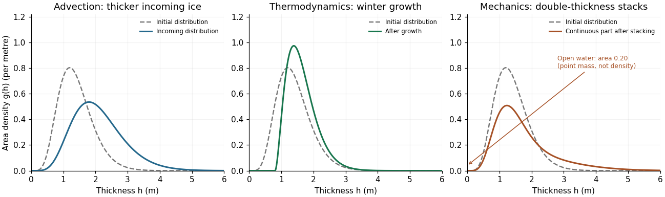
The figure uses illustrative distributions, not measured data. The advection panel compares local ice with incoming thicker ice; the growth panel applies the thickness-characteristic formula; the mechanical panel uses and shows its open-water mass separately from the continuous density.
For the thick tail, take the common-shape sea-ice pressure ridge idealization to mean triangular profile sections with a common effective side slope , while peak thicknesses vary. Let count sea-ice pressure ridge peaks per track length with maximum thickness in . Above a level-ice baseline , a sea-ice pressure ridge with contributes two flank lengths at thickness ; it contributes nothing at . For a representative transect, summing these lengths gives the triangular ridge occupation identitySuppose for . ThenThus an exponential ridge-draft model, expressed in the same vertical coordinate as the profile, generates an exponential occupation tail with the same decay parameter. The peak-count distribution and the area-weighted thickness distribution are different distributions, so their amplitudes carry essential information.
If is ridge line density and is the tail's area fraction, the same result becomesThe decay rate alone does not fix slope: sea-ice pressure ridge frequency or tail amplitude is also needed. If side slopes vary independently of peak height, replace by , giving an effective harmonic-mean slope. Measured along-track slopes differ from slopes normal to a ridge if the transect is oblique. Overlap, irregular shape and porosity limit this simple geometric model. Literally identical complete ridge cross-sections would have one height, so “common shape” here necessarily permits different ridge sizes.
Sea-ice pressure ridge spacings are positive and broadly distributed. A spatial Poisson process gives an exponential distribution of gaps, a useful simple approximation. Observed sea-ice pressure ridge spacings, however, often fit a shifted lognormal distribution better, with few very small spacings because of ridge geometry, identification rules and finite beam width. This differs from the successful exponential model for peak drafts. Observed ridge-spacing and draft distributions establish this distinction.
Sea-ice lead-width distributions contain very many narrow openings and a broad tail. A power law often describes widths over a resolved range better than one negative exponential; its exponents and apparent cutoffs depend on the lead definition, resolution and count-versus-area weighting. Sea-ice lead spacings may be approximately exponential over an intermediate range, but clustering produces excess close pairs and large gaps, so there is no universal independent-spacing law. Both behaviors were found in Greenland Sea and Eurasian Basin lead statistics. Advection imports thickness classes, thermodynamics transports them in , and mechanics exchanges thin-ice area for ridged ice and leads; common-slope exponential ridge populations reproduce the exponential thick tail.
Past exam of the mathematics course of the University of Cambridge 2008 iii Paper 89 2 Solution by Codex 0 Created 2026-10-03 Updated 2026-10-14
Codex 0 Created 2026-10-03 Updated 2026-10-14Let denote ice and snow thickness, let increase downwards, and count external atmospheric fluxes as positive into the surface. The Maykut-Untersteiner model is a time-dependent column model, rather than a single thickness formula: heat conduction, heat storage, internal absorption of sunlight and moving freezing/melting boundaries must be solved together. In an ice-following description its energy equation can be writtenwhere is specific enthalpy, is the prescribed ice salinity, and is the downward penetrating shortwave flux. The material derivative includes coordinate motion if a moving numerical grid is used. A common attenuation form is within a homogeneous ice layer, with the origin taken at that layer's top. The corresponding source is . Snow-covered cases have much less penetration; absorbed surface radiation must not also be counted as internal heating.
The liquid brine fraction contributes latent heat to the effective specific heat capacity: for the illustrative liquidus approximation with Celsius in the mixed-phase range , . The precise ice conductivity and heat capacity are salinity- and temperature-dependent. This is why the full transient temperature profile need not be linear. At the snow-ice interface impose continuity of temperature and conductive heat flux; at the ice bottom impose the seawater freezing temperature .
Write and define the atmospheric input absorbed at the surface byHere is the surface albedo, is the Stefan-Boltzmann constant, and are signed sensible and latent turbulent heat fluxes. With upward conductive flux , the cold, nonmelting surface satisfies . Once the surface reaches its melting temperature, constrain it there and use excess energy for ablation:The mass-loss rate first removes snow at thickness rate ; after the snow is gone it removes ice at rate . Snow thickness also changes through prescribed snowfall and any separately represented compaction or sublimation.
At the bottom, the Stefan condition equates latent heat released by growth to upward conductive removal minus upward ocean heat flux :Here is positive for basal freezing and negative for basal melting, and is the appropriate effective latent heat. These equations, the incident fluxes and snowfall determine the seasonal thickness trajectory. Annual sea-ice thermodynamic equilibrium means a periodic temperature field and , soWith constant , this is equivalently . An “equilibrium thickness” must refer to the mean or a specified phase of this seasonal cycle.
A useful winter reduction neglects heat storage and solar penetration and treats each conductivity as constant. The two layers act as thermal resistances in series:This displays the dependence on snow and ice thickness, but is not a replacement for the full seasonally forced Maykut-Untersteiner model.
Increasing ocean heat flux subtracts directly from basal growth and increases bottom ablation. On a stable perennial branch it lowers annual equilibrium thickness, and sufficiently large input can eliminate a year-round ice cover. With zero oceanic input, removing this heat sink can allow much thicker thermodynamic ice; it does not remove the seasonal surface energy balance.
Additional annual snowfall has competing effects. Larger suppresses winter heat conduction and basal growth, favoring thinner ice. But persistent bright snow raises albedo, consumes energy when it melts and delays exposure of dark bare ice, suppressing summer ice ablation. The original column calculations show near compensation for moderate snowfall and substantial thickening when much more snow survives into summer. Thus annual equilibrium thickness need not decrease with snowfall, even though greater snow thickness at fixed winter temperatures always reduces the conductive growth rate. The balance also depends on snowfall timing and the treatment of snow-to-ice conversion. These seasonal responses are illustrated by the original model calculations.
Reducing surface albedo increases absorbed shortwave radiation. It promotes surface ablation, internal heating and, where sunlight reaches the ocean, basal ablation; the ice-albedo feedback reinforces the reduction in equilibrium ice thickness. Increasing albedo has the opposite effect. This sensitivity is strongest when sunlight is available and dark surfaces are exposed, rather than during polar night.
For the observed bottom melt, use , and approximately 122 days. The basal melt heat flux equivalent isThe integrated latent heat is about . This is energy used for melting, not automatically the complete ocean-to-ice heat input: the basal balance gives , with sensible heat and salinity corrections if needed.
A likely major source is solar heating of an unusually large open-water fraction. Dark water absorbs much more sunlight than snow-covered ice, and warm water transfers that stored heat to floe bottoms by mixing and lateral transport. Thin or ponded ice also transmits more sunlight. Wind-driven divergence and export expose additional water, while advection of warm Pacific or Atlantic water and mixing of subsurface heat can contribute regionally. The supplied melt amount alone cannot partition these sources. The 2007 Beaufort Sea heat-budget analysis found that locally absorbed solar heat was sufficient to account for the enhanced basal melt. The latent-heat equivalent is about ; increased solar absorption by exposed ocean is a well-supported principal explanation.
Past exam of the mathematics course of the University of Cambridge 2008 iii Paper 89 1 Solution by Codex 0 Created 2026-10-03 Updated 2026-10-14
Codex 0 Created 2026-10-03 Updated 2026-10-14In seawater, freezing produces nearly salt-free solid and leaves salt in the interstitial liquid. The growing cover is therefore a mushy layer, with sea-ice crystal fabric determined by both crystal growth and the mechanical history. Crystallographic c-axes are perpendicular to the plates' basal planes; grain elongation and c-axis orientation must not be confused.
For first-year sea ice growing by congelation, heat loss first brings the surface water to its salinity-dependent freezing point. Small frazil ice crystals may form and collect into a thin continuous sheet, or a quiet surface can freeze directly; the resulting nilas provides the initial cover. Once the water surface is protected from strong agitation, heat transported by heat conduction upward through the sheet permits freezing onto its underside. Competitive growth favors grains with fast basal-plane growth directed downward, so grains with approximately horizontal c-axes crowd out less favorably oriented grains. The mature congelation ice consists predominantly of long vertical columns beneath a finer initial surface layer. Within and between these grains, the advancing cellular interface traps brine-bearing spaces. The growth sequence and crystallographic selection explain why the resulting texture is columnar rather than a random aggregate of floating crystals.
For pancake ice, wind and surface gravity waves prevent an uninterrupted ice sheet. Supercooled surface water produces suspended frazil ice; crystals accumulate into grease ice and then small coherent cakes. Wave-induced convergence, collisions and repeated accumulation of frazil increase cake size and thickness. Collisions and overwash deposit slush around the margins, building the characteristic raised rims. The crystal aggregate is predominantly granular, with much less systematic orientation than in congelation ice. A calmer interval can add a columnar basal layer, so a pancake need not be purely granular throughout. Observed pancake structures include frazil layers, basal congelation growth and rafted cakes.
In Antarctic consolidated pancake ice, the active edge initially follows this frazil-pancake route. As concentration rises and waves are attenuated, pancakes jam, raft and become frozen together, with interstitial frazil filling the gaps. The consolidated sheet retains overlapping cake outlines, stacked granular layers and an irregular underside, rather than acquiring the simple fabric of a single quiet-water-grown sheet. Later basal freezing can add congelation ice, but the granular fraction often remains large. Snow loading or overwash can flood the top; freezing this slush adds granular snow ice, a separate contribution from seawater-derived frazil. These mechanisms produce the heterogeneous sea-ice crystal fabric documented in cores from the Antarctic marginal ice zone. Quiet basal growth produces columnar ice; wave-driven aggregation and consolidation produce predominantly granular, layered ice.
The main efficient net desalination mechanisms require transport through the ice boundary. In gravity drainage of sea-ice brine, cold saline liquid is denser than the water below, so a connected permeable pore network permits downward flow and compensating entry of less saline seawater. Dense brine can collect into channels and convective drainage pathways. For a layer of depth , a Darcy law estimate of drainage speed is , giving a drainage time and showing directly why permeability of a porous medium and buoyancy matter. Warm, brine-rich ice drains much more readily than cold ice whose pores have become poorly connected. This is important during growth and can intensify as warming reconnects channels; an isolated sealed brine pocket cannot drain merely because its liquid is dense. The connectivity constraint is supported by sea-ice permeability measurements.
In meltwater flushing of sea ice, water supplied by surface snow melt or melt ponds has a hydraulic head above sea level and percolates down connected pores and cracks, displacing brine. It can remove salt rapidly in warm summer ice. Its limits are the supply and head of meltwater and pore connectivity; lateral runoff may reduce the amount available for vertical flushing. Gravity-driven drainage can act without surface melting, whereas flushing cannot.
Brine expulsion occurs when additional freezing and solid expansion pressurize an inclusion and force liquid into nearby passages. This is often internal redistribution: expelling brine from one inclusion does not desalinate the entire floe unless that liquid reaches the ocean. Migration of brine inclusions involves melting on a warmer wall and refreezing on the colder wall; molecular salt diffusion through liquid connections is also possible. These slow processes are far less effective at exporting bulk salt than connected advective drainage. Diffusion through the ice lattice itself is extremely slow. Likewise, excluding salt from each growing crystal is not by itself proof of salt loss from a whole ice-brine mixture. Desalination experiments and transport calculations distinguish net salt export from internal redistribution. Gravity drainage dominates desalination of permeable growing ice; meltwater flushing can dominate summer desalination; expulsion, inclusion migration and diffusion are comparatively ineffective without a boundary-crossing flow.
Pinned article: Introduction to the OurBigBook Project
Welcome to the OurBigBook Project! Our goal is to create the perfect publishing platform for STEM subjects, and get university-level students to write the best free STEM tutorials ever.
Everyone is welcome to create an account and play with the site: ourbigbook.com/go/register. We belive that students themselves can write amazing tutorials, but teachers are welcome too. You can write about anything you want, it doesn't have to be STEM or even educational. Silly test content is very welcome and you won't be penalized in any way. Just keep it legal!
Intro to OurBigBook
. Source. We have two killer features:
- topics: topics group articles by different users with the same title, e.g. here is the topic for the "Fundamental Theorem of Calculus" ourbigbook.com/go/topic/fundamental-theorem-of-calculusArticles of different users are sorted by upvote within each article page. This feature is a bit like:
- a Wikipedia where each user can have their own version of each article
- a Q&A website like Stack Overflow, where multiple people can give their views on a given topic, and the best ones are sorted by upvote. Except you don't need to wait for someone to ask first, and any topic goes, no matter how narrow or broad
This feature makes it possible for readers to find better explanations of any topic created by other writers. And it allows writers to create an explanation in a place that readers might actually find it.
Figure 1. Screenshot of the "Derivative" topic page. View it live at: ourbigbook.com/go/topic/derivativeVideo 2. OurBigBook Web topics demo. Source. - local editing: you can store all your personal knowledge base content locally in a plaintext markup format that can be edited locally and published either:This way you can be sure that even if OurBigBook.com were to go down one day (which we have no plans to do as it is quite cheap to host!), your content will still be perfectly readable as a static site.
- to OurBigBook.com to get awesome multi-user features like topics and likes
- as HTML files to a static website, which you can host yourself for free on many external providers like GitHub Pages, and remain in full control

Figure 2. You can publish local OurBigBook lightweight markup files to either OurBigBook.com or as a static website.
Figure 3. Visual Studio Code extension installation.
Figure 5. . You can also edit articles on the Web editor without installing anything locally. Video 3. Edit locally and publish demo. Source. This shows editing OurBigBook Markup and publishing it using the Visual Studio Code extension. 
- Infinitely deep tables of contents:



All our software is open source and hosted at: github.com/ourbigbook/ourbigbook
Further documentation can be found at: docs.ourbigbook.com
Feel free to reach our to us for any help or suggestions: docs.ourbigbook.com/#contact