With , the Gauss-Seidel method solves . It uses each newly computed coordinate immediately in the remaining triangular solve. It is successive over-relaxation with parameter one, and converges from every start when is a symmetric positive-definite matrix.
To solve a linear system , split its matrix into the diagonal matrix and the strictly lower and upper parts , retaining their actual signs. Every diagonal entry must be nonzero. A sweep updates coordinates in order:The Jacobi method uses the old vector throughout; the Gauss-Seidel method reuses each fresh coordinate. Thus the update order is part of the method.[ref]
Notes for Ma221 Lecture 21, Nov 10 2009. Math 221, Matrix Computations, Fall 2009; Gauss-Seidel: component loop, splitting and update-order remark, web lines 372–380
The matrix splitting has , , so its iteration matrix isCompute the update by forward substitution with the lower triangular matrix , rather than forming a matrix inverse. For a sparse matrix, a sweep only visits stored entries and can overwrite the working vector. Dependencies on fresh coordinates constrain parallel execution. This makes the Gauss-Seidel method an inexpensive solver component, including in a multigrid method.[ref]
Notes for Ma221 Lecture 21, Nov 10 2009. Math 221, Matrix Computations, Fall 2009; Basic iterative methods, cheap splitting requirement; Gauss-Seidel loop and red-black ordering; opening list of solver building blocks
For a real symmetric positive-definite matrix , let be the Gauss-Seidel method error and . Its recurrence gives . Expanding the two squared energy norms yields . Every diagonal entry of is positive, so the error energy strictly decreases unless . In that case and the exact solution has already been reached. This identity exhibits the method as a sequence of energy-reducing coordinate corrections.
Consider the original linear systemDirect substitution verifies the solution. The matrix is a symmetric positive-definite matrix: completing the square in its quadratic form gives for every nonzero vector. It is also a strictly diagonally dominant matrix.
Starting from , update the first row and then the second:The first sweep gives and . The next gives and . The second row uses during the first sweep, even though the initial first coordinate was zero.
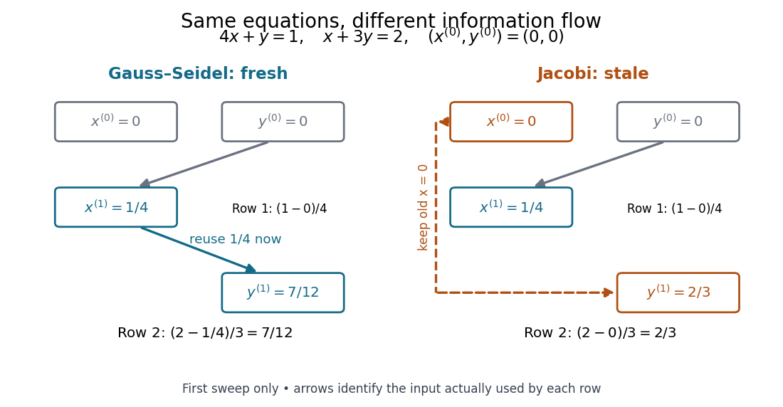
Fresh and stale inputs in the first sweep of the original two-variable linear system
. Details. With a stale first coordinate, the Jacobi method would instead give after the first sweep. Both methods have the same fixed point, but changing when coordinates become available changes the entire sequence of vectors.
For the Gauss-Seidel iteration for a two-variable positive-definite system, define the forward error by and . Subtract the two exact solution equations from the two update equations:The fresh first coordinate passes the old second-coordinate error through two successive factors. The iteration matrix is thereforeIts eigenvalues are and , as seen from the determinant. The zero eigenvalue explains why the old first-coordinate error disappears completely: the first row overwrites it. After one sweep, every remaining forward error lies on the eigenvector line spanned by .
For this zero start, , so the exact vectors for areThe Euclidean norm of the forward error decreases by exactly per sweep from onward. The first decrease is different because the initial error has not yet reached that eigenvector line. Each row update moves horizontally or vertically in the coordinate plane; sweep endpoints then approach the solution along one straight line.
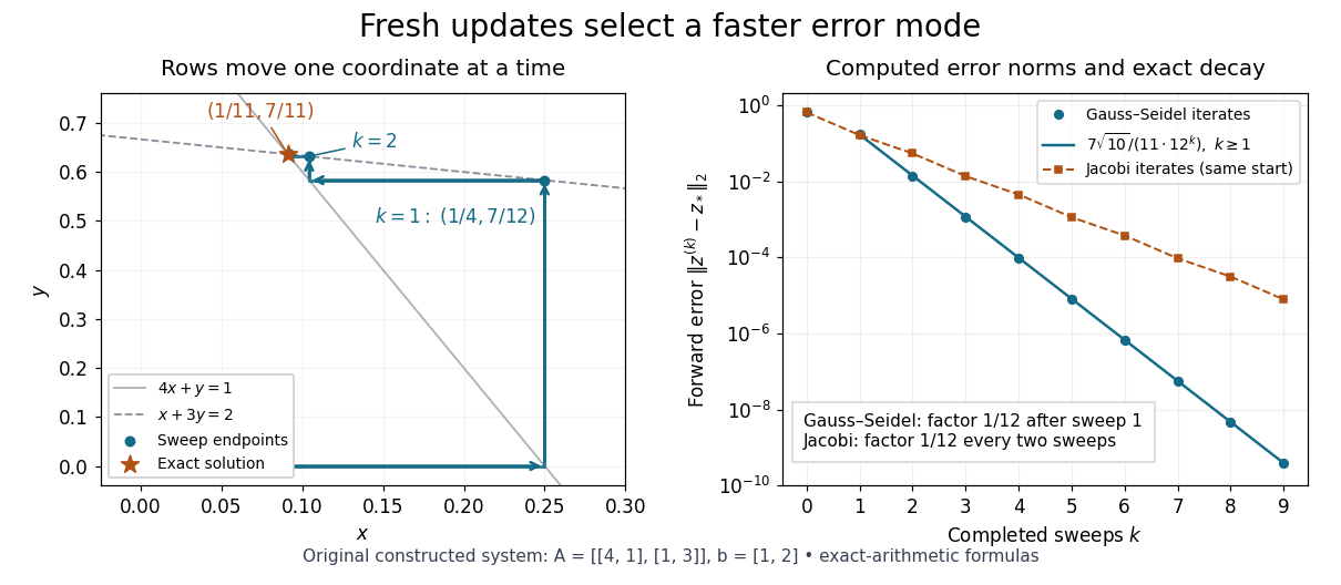
Computed row-by-row Gauss-Seidel method trajectory and exact forward error contraction for the original two-variable linear system
. Details. The linear-system residual is an independent way to check the calculation. Completing a sweep satisfies the second row exactly, but changing disturbs the first row:Thus a zero residual in the last updated row alone does not certify a solution; inspect the complete linear-system residual.
For the same matrix, the stale schedule of the Jacobi method gives the iteration matrixHere its eigenvalues are , whereas the fresh schedule gives . This comparison belongs to this particular linear system; it is not a universal relation between the two methods' spectral radii.
A strictly diagonally dominant matrix or a real symmetric positive-definite matrix guarantees convergence of the Gauss-Seidel method from every initial vector. These are sufficient conditions.[ref]
Notes for Ma221 Lecture 21, Nov 10 2009. Math 221, Matrix Computations, Fall 2009; Theorem 1, strict row diagonal dominance, web lines 462–465; Theorem 3, positive-definite SOR and its ω = 1 specialization, web lines 490–493
For strict diagonal dominance, putInduct through a sweep. Old coordinates have absolute error at most ; previously updated coordinates have absolute error at most . The component update and the triangle inequality therefore bound the new error by . This proves , a maximum norm contraction.
For a symmetric positive-definite matrix, write . The Householder-John theorem applies to and , because is a positive-definite matrix. Hence the iteration matrix has spectral radius less than one, which gives the convergence criterion for a stationary iteration.
There is also a geometric reason fresh updates help: the Gauss-Seidel method is exact coordinate descent on the convex quadratic functionHolding the other coordinates fixed, minimizing in coordinate gives the corresponding row update. A change lowers by exactly . Each fresh coordinate is therefore the minimizer for the current vector, and a complete sweep lowers the quadratic form error unless every coordinate already solves its row. This explains the method's beauty without implying monotone decrease in every vector norm.
An invertible matrix and nonzero diagonal entries make the update well defined, but do not guarantee convergence. For the original linear systemthe Gauss-Seidel method updates and . Starting at zero gives , then . The second-coordinate forward error is , and the iteration matrix has spectral radius . The linear system has a unique solution while this particular stationary iterative method for a linear system diverges.
Articles by others on the same topic



The Gauss-Seidel method is an iterative technique used to solve a system of linear equations of the form \(Ax = b\), where \(A\) is a matrix, \(x\) is the vector of unknowns, and \(b\) is the output vector. This method is particularly useful for large systems where direct methods like Gaussian elimination might be computationally expensive.