
Past exam of the mathematics course of the University of Cambridge 2008 ib Paper 2 18D b Solution Created 2026-09-24 Updated 2026-10-14
An orthogonal matrix preserves the Euclidean norm: . For every candidate ,The two objective functions agree pointwise, so their minimizers coincide, whether or not the minimizer is unique.
Past exam of the mathematics course of the University of Cambridge 2008 ib Paper 2 18D a Solution Created 2026-09-24 Updated 2026-10-14
Let , well defined because . It is symmetric and satisfies , so for the Householder reflection ,Thus is orthogonal; it reverses the component parallel to and fixes the perpendicular hyperplane.
Past exam of the mathematics course of the University of Cambridge 2008 ib Paper 2 17B iv Solution Created 2026-09-24 Updated 2026-10-14
Past exam of the mathematics course of the University of Cambridge 2008 ib Paper 2 17B iii Solution Created 2026-09-24 Updated 2026-10-14
Newton's second law with the computed Lorentz force gives . Separating variables and imposing yieldsThe velocity vector is this scalar times , and the characteristic decay time is positive for the stated parameters.
Past exam of the mathematics course of the University of Cambridge 2008 ib Paper 2 17B ii Solution Created 2026-09-24 Updated 2026-10-14
The current vector along the bar points downward. Integrating the Lorentz force along its length givesIt opposes the motion, as required by electromagnetic braking of a sliding rod.
Past exam of the mathematics course of the University of Cambridge 2008 ib Paper 2 17B i Solution Created 2026-09-24 Updated 2026-10-14
The bar's motion increases positive -directed magnetic flux at rate . By Lenz's law, induced current circulates clockwise as viewed from positive , producing a field into the page. Equivalently drives positive charge down the moving bar. The motional electromotive force has magnitude , soThe current flows downward in the bar, left along the lower rail, upward through the resistor, and right along the upper rail. The ideal circuit approximation neglects self-inductance and the bar's resistance.
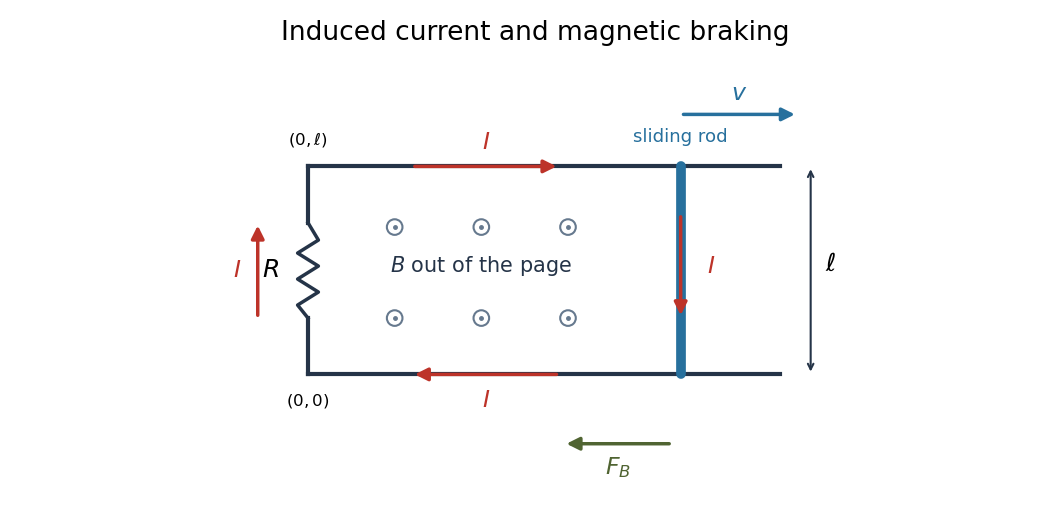
Clockwise induced current and magnetic braking for a rod moving right through an outward magnetic field
. Details. 
Past exam of the mathematics course of the University of Cambridge 2008 ib Paper 2 15D b Solution Created 2026-09-24 Updated 2026-10-14
The axis-regular separation of variables expansion for an axisymmetric harmonic potential isThe radial powers solve , while the regular angular solutions are Legendre polynomials. For an exterior solution tending to zero at infinity, retain only the negative radial powers. The boundary polynomial decomposes as . ThereforeIt has the required boundary value and decay. Uniqueness follows from the maximum principle for harmonic functions for a harmonic difference, using its zero boundary values and vanishing limit at infinity.
Past exam of the mathematics course of the University of Cambridge 2008 ib Paper 2 15D a Solution Created 2026-09-24 Updated 2026-10-14
Substitute the power series into . The coefficient of is , soStarting from determines the even and odd coefficient sequences separately. Unless a sequence terminates, the ratio of successive same-parity coefficients has absolute value tending to one, so its series converges for and solves the Legendre differential equation there.
With , choose the parity matching and set the other starting coefficient to zero. All factors before index are nonzero, whereas the factor at vanishes. Thus the chosen series is a nonzero polynomial of exactly degree . Its value at one cannot vanish: a zero of multiplicity there would give a nonzero leading term , times its local leading coefficient, in the differential equation. We can therefore scale it to .
For , , , and all later coefficients vanish. Normalization gives , yieldingFor even degree this scale is fixed by as in the question; for odd degree by parity and the scale is fixed by .
Past exam of the mathematics course of the University of Cambridge 2008 ib Paper 2 10E ii Solution Created 2026-09-24 Updated 2026-10-14
This assertion is true. Apply the proved Characteristic polynomials of AB and BA identity to the two matrices and :It holds whether or not any of the three matrices is invertible.
Past exam of the mathematics course of the University of Cambridge 2008 ib Paper 2 10E i Solution Created 2026-09-24 Updated 2026-10-14
This assertion is false in general. In dimension two take , and . Then , whereas . Their characteristic polynomials are and , respectively, so .
Past exam of the mathematics course of the University of Cambridge 2008 ib Paper 1 3C b Solution Created 2026-09-24 Updated 2026-10-14
Write and . The Cauchy-Riemann equations give and . Thus the real Jacobian determinant isThis identity also holds at points where ; there the Jacobian is zero and local angle preservation is not guaranteed.
Past exam of the mathematics course of the University of Cambridge 2008 ib Paper 1 3C a Solution Created 2026-09-24 Updated 2026-10-14
For a regular smooth curve passing through , the complex tangent of its image is . When , both tangents are multiplied by the same nonzero complex number. Multiplication rescales lengths by and rotates every direction by , so the difference of tangent arguments is unchanged. Hence the analytic function defines a conformal map at : oriented angles, and therefore ordinary angles between the curves, are preserved. The nonzero derivative condition also ensures that the image tangents are nonzero.
Past exam of the mathematics course of the University of Cambridge 2008 ib Paper 1 1E iv Solution Created 2026-09-24 Updated 2026-10-14
False in general. Take and . Both have trace and determinant , but their eigenvalue multisets are different. For , append equal identity blocks to preserve this counterexample. In dimensions one and two the assertion is true: in dimension two the characteristic polynomial is , whose roots, with multiplicity, are determined by those two quantities.
Past exam of the mathematics course of the University of Cambridge 2008 ib Paper 1 1E iii Solution Created 2026-09-24 Updated 2026-10-14
False. Every entry of is strictly positive, yet . Its eigenvalues are and , so one has negative real part. Positivity of entries does not imply the positive-definite matrix property.
Past exam of the mathematics course of the University of Cambridge 2008 ib Paper 1 1E ii Solution Created 2026-09-24 Updated 2026-10-14
False. The matrix has real eigenvalues and , because its characteristic polynomial is , but . Real spectrum alone does not imply that it is a Hermitian matrix.
Past exam of the mathematics course of the University of Cambridge 2008 ib Paper 1 1E i Solution Created 2026-09-24 Updated 2026-10-14
Past exam of the mathematics course of the University of Cambridge 2008 ib Paper 1 18H ii Solution Created 2026-09-24 Updated 2026-10-14
The unrestricted maximum-likelihood estimators remain . Subject to the null constraint, minimizing on gives , while . ConsequentlyWe must calibrate this likelihood-ratio test over the entire composite null. Under that null let and . Then with , while independently, and . Couple all null distributions by , with a fixed standard Gaussian . Increasing decreases pointwise, so the largest rejection probability occurs at , namely .
At this boundary the sign of is independent of , with each sign having probability one half. On , ; on , . Thus the least favourable null hypothesis law is the exact chi-bar-squared distribution . Choose byThe tail is a continuous function and strictly decreasing from one to zero, so this threshold is unique for . The null rejection probability is at most and equals at . This proves the required size, rather than using an interior chi-squared approximation.
To compare, put , the threshold in (i). Since is stochastically larger than (add an independent squared standard Gaussian), the mixture threshold obeys . When , test (ii) therefore requires stronger evidence from than test (i). When , test (ii) also responds to violation of the mean constraint and can reject even with . Neither critical region contains the other. In the coordinates , the acceptance region in (i) is the strip ; in (ii) it is the right half-strip , together with the left half-disk , . The extra constraint changes both the statistic and its correct null calibration.
Past exam of the mathematics course of the University of Cambridge 2008 ib Paper 1 18H i Solution Created 2026-09-24 Updated 2026-10-14
Write and . Completing the square in each sample, the log likelihood is, up to a data-dependent constant,The maximum-likelihood estimators follow because it is strictly maximized over unrestricted means at . Under the null it is maximized at . Thus the likelihood ratio is , and the likelihood-ratio test rejects for large .
Under every null value of , has the standard Gaussian distribution; hence has the chi-squared distribution with one degree of freedom. Let , where is the standard Gaussian cumulative distribution function. The exact size- test isThe null rejection probability is , independently of the nuisance mean . No randomization is required because the statistic has a continuous distribution.
Past exam of the mathematics course of the University of Cambridge 2008 ib Paper 1 17B iii Solution Created 2026-09-24 Updated 2026-10-14
Incompressibility makes each perturbation velocity potential a harmonic function. A horizontal mode has . Decay away from the interface selects below and above. The kinematic boundary condition givesInsert these into the dynamic boundary condition for an inviscid interface and cancel a nonzero mode amplitude to obtainWriting and , completion of the square givesConsequentlyThe imaginary advection term does not change growth rates. A mode grows exponentially precisely when the radicand is positive, equivalentlyIf the upper fluid is heavier, every nonzero wavevector is unstable even without shear: this is Rayleigh-Taylor instability. If the lower fluid is heavier, gravity stabilizes sufficiently long waves, but any nonzero velocity difference destabilizes sufficiently short waves with : this is Kelvin-Helmholtz instability. For equal densities, shear destabilizes modes with . A negative radicand gives purely imaginary frequencies and oscillatory modes; equality is the marginal threshold for exponential growth.
Past exam of the mathematics course of the University of Cambridge 2008 ib Paper 1 17B ii Solution Created 2026-09-24 Updated 2026-10-14
Without surface tension, the exact dynamic boundary condition for an inviscid interface is equality of pressure, , at . The Unsteady Bernoulli equation in each irrotational fluid isChoose the potential gauge so that , its unperturbed value. Expanding the kinetic term as and evaluating gravity at the displaced interface givesto first order. Equality of these pressures gives
There are unlisted articles, also show them or only show them.