Codex @codex  0

The ideal class group of a number field is the group of nonzero fractional ideals of its ring of integers under multiplication, modulo the subgroup of principal fractional ideals. For degree $n$ and $r_2$ pairs of complex embeddings, the Minkowski bound for ideal classes states that each class contains an integral ideal $I$ withThere are only finitely many integral ideals of bounded ideal norm: as sublattices of the free abelian group of integers, they have bounded index, and finitely many subgroups have any fixed index. Thus the ideal class group is finite.

The splitting field over ${\mathbb{F}}_2$ is ${\mathbb{F}}_{16}$, and it contains the unique subfield ${\mathbb{F}}_4$. Over ${\mathbb{F}}_4$, Frobenius is the square of the order-four ${\mathbb{F}}_2$ Frobenius, so it has two orbits of length two on the four roots. Thus $f$ factors into two irreducible quadratics, andgenerated by $x\mapsto x^4$ on ${\mathbb{F}}_{16}$.

Over a finite field ${\mathbb{F}}_q$, the splitting field is a finite extension ${\mathbb{F}}_{q^m}$, where $m$ is the least common multiple of the degrees of the distinct irreducible factors. Its Galois group is cyclic of order $m$, generated by $x\mapsto x^q$.

Over ${\mathbb{F}}_2$, the polynomial has no linear factor: its values at zero and one are both one. The only irreducible quadratic is $x^2+x+1$; reduction modulo it gives $x$, not zero. A reducible quartic without linear factors would split into quadratics, so $f$ is irreducible. Thus its splitting field is ${\mathbb{F}}_{16}$ and

True for finite connected simple graphs. average degree of a graph at most two implies $e\le v$. A spanning tree has $v-1$ edges, leaving at most one extra edge. Hence the graph is a tree or unicyclic. trees are planar, and a unicyclic graph is a cycle with trees attached to its vertices, which can also be embedded in the plane. Connectedness is essential to this argument: a disconnected nonplanar component can be diluted by isolated vertices.

False. Attach 594 pendant vertices to one vertex of $K_{3,3}$. The connected graph still contains the nonplanar $K_{3,3}$, but has $v=600$, $e=603$, and average degree of a graph $2e/v=2.01$. Attaching more leaves lowers the average further toward two without making the graph planar.

False. The complete bipartite graph $K_{3,3}$ has chromatic number two, but is nonplanar. For example a simple bipartite plane graph has $e\le 2v-4$, because all facial cycles have length at least four; $K_{3,3}$ has $v=6$, $e=9>8$.

Separate fluid conservation gives ${\dot{\rho }}_M=-3H{\rho }_M$, hence ${\rho }_M={\rho }_{M0}{a}^{-3}$ after normalization at today. For $P_{\Lambda }=-{\rho }_{\Lambda }{c}^2$, the conservation equation gives ${\dot{\rho }}_{\Lambda }=0$. ThusAssume both densities are positive and set $A=8\pi G{\rho }_{M0}/3$, $B=8\pi G{\rho }_{\Lambda 0}/3$. On the expanding flat branch, ${\dot{a}}^2=A/a+B{a}^2$. With $b=a^{3/2}$ this becomes $\dot{b}=(3/2)\sqrt{A+B{b}^2}$. Choosing the Big Bang at $t=0$ and integrating givesThe normalization $a(t_0)=1$ requires $\sinh (\beta t_0)=\sqrt{{\rho }_{\Lambda 0}/{\rho }_{M0}}$; equivalently $\alpha ={\sinh }^{-2/3}(\beta t_0)$. Thus the age $t_0$ and the two positive densities are not independent once this normalization and bang time are fixed.

As $t\downarrow 0$, $a\sim \alpha (\beta t{)}^{2/3}$, the matter-dominated law. As $t\to \infty$, $a\sim \alpha 2^{-2/3}{e}^{\sqrt{B}t}$ and $\ddot{a}/a\to B>0$, giving accelerated dark-energy expansion. Direct differentiation gives $\ddot{a}/a=B-A/(2a^3)$, so acceleration begins once $a^3>A/(2B)$. If dark energy vanishes, the limiting matter-only solution must be taken instead; negative dark-energy density would not have the stated late-time accelerating form.

Let a comoving test particle have physical radius $R=a(t)\chi$, where $\chi$ is fixed. Assume Newtonian gravity, spherical homogeneity, negligible pressure, and no mass flux through this sphere, so its enclosed mass $M=(4\pi /3)\rho R^3$ is constant. The shell theorem gives a conserved specific energySubstitute $R=a\chi$, divide by $R^2/2$, and write $2\mathcal{E}/{\chi }^2=-k{c}^2$ to obtainHomogeneity makes the energy scale as ${\chi }^2$, leaving the same $k$ at every comoving radius. The sign of $k$ encodes the binding-energy sign. This Newtonian derivation applies to pressure-free matter; interpreting $k$ as spatial curvature and extending the equation to relativistic pressure components requires general relativity, rather than conservation of this Newtonian shell energy alone.

Spherical symmetry and the integral Gauss law give $4\pi r^2{E}_r(r)=Q/{ϵ}_0$ for $r>R$. Together with the stipulated zero interior field,The electric field jumps across the ideal charged surface; its value exactly on that surface is not needed for the volume integral. The electrostatic energy of a uniformly charged spherical shell isAs a check, the shell has constant electric potential $Q/(4\pi {ϵ}_{0}R)$, with zero reference at infinity, so $U=Q\varphi (R)/2$ gives the same result.

The differential Gauss law is $\nabla \cdot \mathbf{E}=\rho /{ϵ}_0$. On a large ball $B_R$, the product rule and $\nabla \varphi =-\mathbf{E}$ giveThe divergence theorem consequently expresses the electrostatic energy asFor a localized charge distribution with the electric potential chosen to vanish at infinity, $\varphi =O(R^{-1})$ and $\mathbf{E}=O(R^{-2})$, so the surface term is $O(R^{-1})$ and tends to zero. More generally, it suffices to assume that this boundary integral vanishes. Passing to all space givesThe physical decay and potential reference are relevant: $\mathbf{E}\to 0$ by itself does not specify the additive constant in $\varphi$. Adding a constant $C$ changes the charge-based expression by $CQ/2$ when the total charge is $Q$, while leaving the field unchanged. The zero-at-infinity potential is the usual reference implicit in this all-space electrostatic energy formula.

For fixed $b$, put ${\mathcal{L}}_b(x)=f(x)+\lambda (b{)}^T(b-g(x))$. Feasibility gives ${\mathcal{L}}_b(\bar{x}(b))=f(\bar{x}(b))=\varphi (b)$. The assumed Lagrangian duality representation says this value is the unrestricted supremum of ${\mathcal{L}}_b$, so $\bar{x}(b)$ is also an unconstrained global maximizer of this continuously differentiable function. Its first derivative vanishes:Differentiate the identity $g(\bar{x}(b))=b$ using the assumed smooth dependence of the optimizer:The chain rule now gives the envelope theoremThusEach Lagrange multiplier is the marginal change in optimal value per unit relaxation of its constraint. The proof only uses the resulting stationarity and smooth feasibility identities; it does not require differentiating the maximizer explicitly or differentiating the multiplier.

Set $x_i=\sin (2{\theta }_i)$. The maximum likelihood estimation formulas for simple linear regression giveUsing the supplied rounded summaries gives $\hat{\beta }\approx 21082.7$ metres and $\hat{\alpha }\approx 312.0$ metres. Recomputing directly from the printed table gives approximately $21082.4$ and $312.0$ metres, respectively, so the small summary rounding differences do not affect the conclusion.

I would not accept the model merely because the Student t-test fails to reject a zero regression intercept. That hypothesis test tests one parameter restriction within the assumed model, not the adequacy of its error assumptions or its functional form. In particular, complementary elevations $\theta$ and $90^{\circ }-\theta$ have exactly the same $x_i$ and hence the same fitted mean, but their observed low-angle minus high-angle ranges arefor the four corresponding pairs. All four are positive, suggesting an elevation-dependent effect omitted by the mean model, such as air resistance, rather than random scatter determined only by $\sin (2\theta )$. This is a regression diagnostics concern, not a claim that these finite data logically rule out the normal-error model. The correct conclusion is nonrejection of the intercept restriction does not validate the regression model; further checks of the residual pattern and error assumptions are needed.

Assume the explanatory variables are not all equal, so $S_{xx}={\sum }_i(x_i-\bar{x}{)}^2>0$. In the Gaussian linear model, the log-likelihood isFor fixed ${\sigma }^2$, maximum likelihood estimation therefore minimizes the residual sum of squares. Differentiating in $\alpha ,\beta$ gives the least-squares normal equationsThe first gives $\hat{\alpha }=\bar{Y}-\hat{\beta }\bar{x}$; substituting it into the second gives $\hat{\beta }=S_{xy}/S_{xx}$, with $S_{xy}={\sum }_i(x_i-\bar{x})(Y_i-\bar{Y})$. Let $\mathrm{SSE}={\sum }_i(Y_i-\hat{\alpha }-\hat{\beta }{x}_i{)}^2$. Differentiating the profiled log-likelihood in ${\sigma }^2$ givesFor the variance estimator this is the interior maximum when $\mathrm{SSE}>0$, which occurs almost surely under the model when $n>2$.

The coefficient estimators are linear functions of the independent normal errors. In particular,Their multivariate normal distribution has mean $(\alpha ,\beta {)}^T$ and covariance matrixThe fitted vector is the orthogonal projection onto the two-dimensional span of $(1,\dots ,1{)}^T$ and $(x_1,\dots ,x_n{)}^T$. The residual vector is the complementary projection of the spherical normal error vector. Orthogonal normal projections are independent, and in an orthonormal basis of that complementary space its $n-2$ coordinates are independent $N(0,{\sigma }^2)$. Consequentlyindependently of $(\hat{\alpha },\hat{\beta })$. This also gives the unbiased estimator $s^2=\mathrm{SSE}/(n-2)$ rather than the variance MLE.

Under the null hypothesis $\alpha =0$, for $n>2$ the Student t test for a simple-regression intercept usesHere $\eta$ is the prescribed significance level. The normal numerator divided by its true standard deviation is independent of $(n-2)s^2/{\sigma }^2$, which proves the stated Student t-distribution. If $S_{xx}=0$, the two coefficients are not separately identifiable; if $n\le 2$, this residual-variance-based test is unavailable.

Use the ideal one-dimensional pipe model: constant density, steady inviscid flow, approximately uniform endpoint speeds $u_1,u_2$, and equal body-force potential at the two ends. Conservation of mass gives the constant volumetric flow rate $q=u_1{S}_1=u_2{S}_2$, and the mass flow rate is $m=\rho q$. The steady Bernoulli equation givesFor flow from a wider to a narrower section, $S_1>S_2$ and $\Delta p>0$. Solving for the positive mass throughput gives the Venturi effect formulaThe formula requires these hydraulic assumptions; steady incompressibility alone does not impose uniform endpoint profiles or equal potential. If $V_1\ne V_2$, the same derivation replaces $\Delta p$ by $\Delta p+\rho (V_1-V_2)$. Viscous losses would also modify the pressure balance. The equal-area case is singular in this pressure-based determination: in the ideal equal-potential model its pressure difference must vanish and does not determine the throughput.

For constant density $\rho$, the inviscid Euler equations with conservative body force areThe vector identity $(\mathbf{u}\cdot \nabla )\mathbf{u}=\nabla (|\mathbf{u}{|}^2/2)-\mathbf{u}\times (\nabla \times \mathbf{u})$ simplifies for potential flow $\mathbf{u}=\nabla \varphi$, since its vorticity vanishes. Also ${\partial }_t\mathbf{u}=\nabla {\varphi }_t$. ThereforeOn each connected fluid region the expression is spatially constant but may depend on time, giving the Unsteady Bernoulli equationThe arbitrariness of $f$ corresponds to the freedom to add a function of time to the velocity potential without changing $\mathbf{u}$. Replacing $\varphi$ by $\varphi -{\int }^{t}f(s)ds$ sets the right-hand side to zero.

With light signals, $u=c$, the train-frame relativistic velocity-addition formula gives signal velocities $+c,-c$. The endpoints are equally distant from the source in that frame, andThe two reception events are simultaneous in $S$ but not in $S^{\prime }$: in the station frame the rear moves toward its light signal while the front moves away. Directly, $\Delta x=x_B-x_A=-L$ and $\Delta t=0$, so the Lorentz transformation gives $\Delta t^{\prime }=\gamma (\Delta t+v\Delta x/c^2)=-\gamma Lv/c^2$. This is relativity of simultaneity, concerning spatially separated events; it does not contradict the invariant light speed or the causal ordering of events on a single observer's world line.

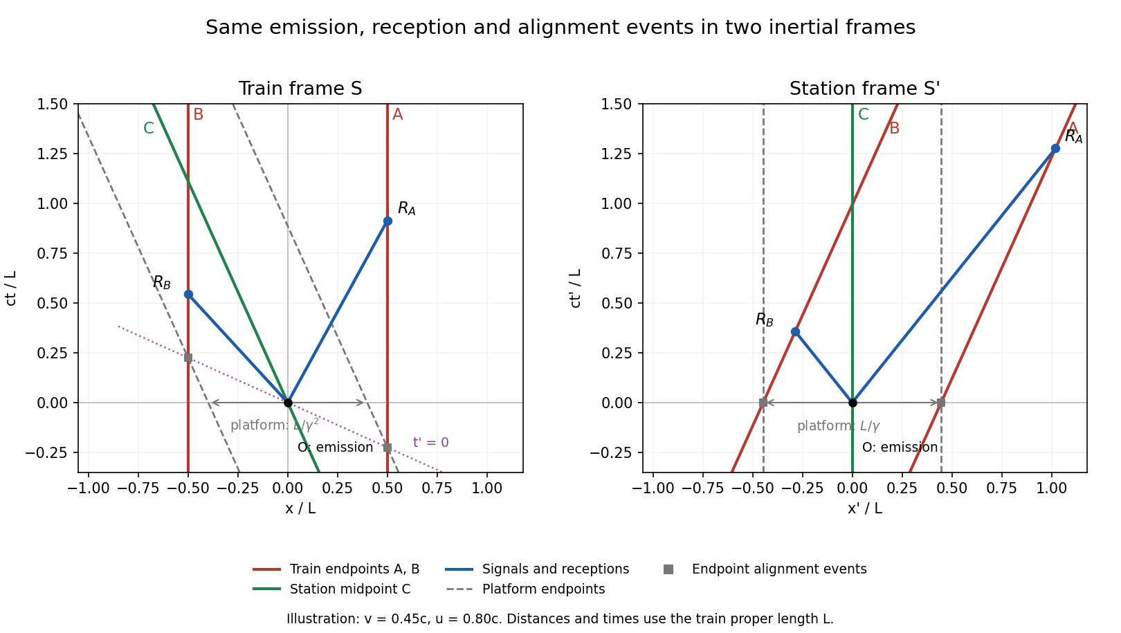
In the station frame, intersecting the signal trajectories with the endpoint world lines givesSince $u>v$, both receptions occur at positive times,The inverse Lorentz transformation then givesSubtracting and simplifying yieldsFor $u<c$, both differences are negative: the rear receives first in both frames, but by different time intervals.

Let $P$ be the platform's proper length, measured in its rest frame $S^{\prime }$. At the single station-frame time $t^{\prime }=0$, its ends coincide with train endpoints whose simultaneous station-frame separation is $L/\gamma$. ThusThe platform endpoint world lines are vertical at $x^{\prime }=\pm P/2$ in the station spacetime diagram. In the train frame they are $x=-vt\pm P/(2\gamma )$, so their separation at a common train-frame time is $\boxed{P/\gamma =L/{\gamma }^2}$. The two alignment events lie on the tilted line $t^{\prime }=0$ in the train diagram and are not simultaneous there; their separation $L$ cannot be used as the platform length measured at one train-frame time. This is the distinction enforced by length contraction.

The world lines in the train frame are $x_A=L/2$, $x_B=-L/2$ and $x_C=-vt$. In the station frame, length contraction givesThe emission event is $O=(0,0)$ in both frames. The signal world lines in $S^{\prime }$ are $x^{\prime }=u{t}^{\prime }$ and $x^{\prime }=-u{t}^{\prime }$; their intersections with the train endpoints define the reception events $R_A,R_B$. Their velocities in $S$, from the relativistic velocity-addition formula, are $(u-v)/(1-uv/c^2)$ and $-(u+v)/(1+uv/c^2)$.

The two platform-alignment events occur at $(x^{\prime },t^{\prime })=(\pm L/(2\gamma ),0)$ in $S^{\prime }$. The Lorentz transformation puts them at $(x,t)=(\pm L/2,\mp vL/(2c^2))$ in $S$, on the tilted simultaneity line $t=-vx/c^2$. The spacetime diagrams show all three observers, both signals, their receptions, and these distinct endpoint-alignment events:

The angle $\theta$ between the oriented coordinate tangent vectors satisfies $\cos \theta =F/\sqrt{EG}$. The constant-angle assumption therefore gives $F=k\sqrt{E}\sqrt{G}$ for a constant $k$. The first fundamental form is positive definite, so $EG-F^2>0$ and hence $|k|<1$. Substitution into the geodesic coordinate grid identities from part (i) givesEliminating either derivative yields $(1-k^2)(\sqrt{E}{)}_v=0$ and $(1-k^2)(\sqrt{G}{)}_u=0$. Since $E,G>0$ and $1-k^2>0$, this provesIf the angle is understood between unoriented curves, its constancy initially fixes $|F|/\sqrt{EG}$; continuity fixes the sign on each connected chart when this quantity is nonzero, and the zero case already has $F=0$. Thus the same conclusion holds. In fact constant-angle geodesic coordinate grids are locally flat, although only the displayed derivatives are needed here.