
Past exam of the mathematics course of the University of Cambridge 2003 ia Paper 3 5E b Solution Created 2026-09-24 Updated 2026-10-14
Put and decompose it into axial and perpendicular parts, . For the nondegenerate semi-angle , the equation is equivalent toThus each plane perpendicular to at axial distance from meets the surface in a circle of radius . Both signs of are allowed, and gives the vertex. This proves that it is a double circular cone with the specified vertex and axis; is the angle each generator makes with either direction of the axis.
For the intersection calculation, define the symmetric matrix . The two equations are . Their difference givesWith and , symmetry of makes the last two terms . Hence the intersection plane of parallel congruent double cones isThe unnormalized normal vector is . Expanding its squared norm givesEquivalently, if , this is . Thus normalization is legitimate and yieldsThe assumption of a genuine cone matters: at the degenerate limits or , the surface collapses respectively to an axis or a plane and this normal need not exist.
Past exam of the mathematics course of the University of Cambridge 2003 ia Paper 3 5E a Solution Created 2026-09-24 Updated 2026-10-14
Move the origin to the centroid and write the four vertex vectors as . Their sum is zero. The midpoints of the first opposite-edge pair have vectors and , so their distances from the centroid are equal. The same argument applies to the other two opposite-edge pairs.
Choose the three midpoint distances as , , . Expanding the dot products,Identifying these four norms with the vertex distances proves the tetrahedron centroid-to-midpoint sum of squares:The proof uses no orthogonality or regularity assumption on the tetrahedron.
Past exam of the mathematics course of the University of Cambridge 2003 ia Paper 3 11A b Solution Created 2026-09-24 Updated 2026-10-14
Take to be continuously differentiable everywhere on , as in the question. Its zero curl says . Construct a potential of a conservative vector field explicitly byAll segments lie in . Differentiating under the integral and using the symmetry of the derivatives,Hence . This radial integral potential for a curl-free field also works on a star-shaped domain after translating its centre. On an arbitrary domain, zero curl only guarantees local potentials; the everywhere-on- interpretation is important for this global assertion.
For the given field, put . The three pairs of derivatives entering its curl areThus the field is irrotational. To find its potential using , integrate to get . Comparison with gives , and comparison with gives . ThereforeDifferentiating this expression reproduces all three components with the required minus sign; the only freedom on the connected domain is the additive constant.
Past exam of the mathematics course of the University of Cambridge 2003 ia Paper 3 11A a Solution Created 2026-09-24 Updated 2026-10-14
Use suffix notation, summing repeated indices. The contraction of two Levi-Civita symbols givesAdding the directional derivative cancels the second term. Interchanging gives another pair whose sum is . The total right-hand side is thereforethe th component of the gradient of the dot product. Since this holds for each component, the dot-product gradient identity is proved:It holds for any continuously differentiable vector fields; no irrotationality assumption is used.
Past exam of the mathematics course of the University of Cambridge 2003 ia Paper 2 7D ii Solution Created 2026-09-24 Updated 2026-10-14
The second component is resonant. Differentiating supplies the term missing from the exponential ansatz:Thus a particular integral isThe linearly growing oscillatory envelope is forced resonance in a differential equation; it does not contradict bounded oscillation of the complementary function. The worked initial-value solution in the question's root Solution uses this same resonant mechanism.
Past exam of the mathematics course of the University of Cambridge 2003 ia Paper 2 7D i Solution Created 2026-09-24 Updated 2026-10-14
Try a particular integral along each forcing eigenvector. Since ,With both denominators nonzero, add the two responses:Only the forcing component's own eigenvalue enters its denominator; a frequency matching a different eigenmode does not create resonance in this already diagonal forcing component.
Past exam of the mathematics course of the University of Cambridge 2003 ia Paper 2 5D b Solution Created 2026-09-24 Updated 2026-10-14
After multiplication by , recognize both sides as derivatives:The nontrivial first integral is thereforeIt necessarily depends on the derivative, correcting the printed notation . A second integration giveson the specified interval. Since , . A finite derivative at zero also implies there, forcing . A positive particular solution is consequentlyThe negative of this function is the other sign choice. Near zero, , so the positive branch has and ; the negative branch has derivative .
For the positive branch, . Its second derivative has numerator , multiplied by a positive factor. This numerator is zero at zero and has derivative , so the curve is convex for positive . It starts tangent to and rises without bound as , with . The third panel of the sketch above shows this branch.
Past exam of the mathematics course of the University of Cambridge 2003 ia Paper 2 5D a Solution Created 2026-09-24 Updated 2026-10-14
An integrating factor for a differential one-form makes the multiplied form exact. If , then and . Equality of the mixed partial derivatives yieldsThis is a local compatibility condition under the usual smoothness assumptions.
For the trigonometric equation, where its coefficients are defined and division is legitimate, the slope is . In the first quadrant it is positive, small near either axis and large near the upper-right corner. The direction field below uses normalized line segments, so steep directions remain visible.
Multiplication by givesThus the multiplying function is an integrating factor, and the implicit general solution isIn the larger square, . The positive- curves have positive and are symmetric about the -axis; the negative- curves are their reflections. For , a graph representation iswith endpoints tending to . The interior curve is . The domain boundaries include singular coefficients or zeros of the integrating factor, so these endpoint limits and smooth continuations through describe the regularized relation; they must not be mistaken for additional solutions of the literal original equation at undefined points.
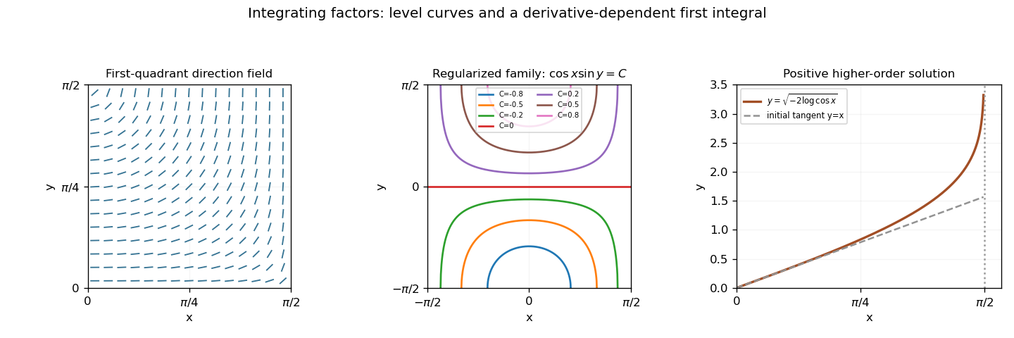
Trigonometric direction field, regularized implicit solution family, and the positive higher-order particular solution
. Details. 
Past exam of the mathematics course of the University of Cambridge 2003 ia Paper 2 3F b Solution Created 2026-09-24 Updated 2026-10-14
For independent random variables, their sum has the product of their probability generating functions:Comparing polynomial coefficients identifies a binomial distribution with parameters :and the probability is zero at all other values. The common success probability is essential to this binomial form; independent binomial counts with different probabilities do not in general add to a binomial count.
Past exam of the mathematics course of the University of Cambridge 2003 ia Paper 2 3F a Solution Created 2026-09-24 Updated 2026-10-14
For a nonnegative integer-valued random variable , its probability generating function isinitially defined at least for . A general real-valued random variable need not have a probability generating function in this sense. For a binomial distribution, the binomial theorem givesDifferentiating the generating function produces factorial moments:Since , the mean and variance areThese formulas include the degenerate endpoint probabilities and .
Past exam of the mathematics course of the University of Cambridge 2003 ia Paper 2 1D ii Solution Created 2026-09-24 Updated 2026-10-14
For , the separated integral isInverting givesThe upper branch has , where decreases towards as . The lower branch has , where decreases to as . These are separate maximal intervals: the pole is not part of a solution. For the domain , a lower-branch initial value below necessarily reaches that pole in finite positive . The direction field sketch above displays both exterior branches and a central hyperbolic tangent branch.
Past exam of the mathematics course of the University of Cambridge 2003 ia Paper 2 1D i Solution Created 2026-09-24 Updated 2026-10-14
Separate variables and integrate on :Hence the general solution in this region isEvery such solution increases from values near towards , remains strictly between the two equilibria, and is defined for all real .
Past exam of the mathematics course of the University of Cambridge 2003 ia Paper 2 10F ii Solution Created 2026-09-24 Updated 2026-10-14
Independence requires each joint probability to equal the product of the relevant marginals. In particular it implies , equivalent to .
Conversely let and , and assume . The covariance calculation gives . ThenAll four joint probabilities therefore factor, proving independence. HenceThis is Bernoulli independence from zero covariance, including degenerate marginals. It is special to two-point variables and is not a general equivalence for arbitrary random variables.
Past exam of the mathematics course of the University of Cambridge 2003 ia Paper 2 10F i Solution Created 2026-09-24 Updated 2026-10-14
The probabilities satisfy and . Since the variables are indicators,Their covariance isThus the necessary and sufficient condition for uncorrelated random variables isThis uses zero covariance as the definition. If one variable is constant, a normalized correlation coefficient is undefined, but zero covariance and this criterion remain meaningful.
Past exam of the mathematics course of the University of Cambridge 2003 ia Paper 1 8D iii Solution Created 2026-09-24 Updated 2026-10-14
For the stated angle, , so . The minimizing unit vector is therefore , andIndeed all three pairwise dot products equal , so the vectors lie in one plane, separated by degrees. This is also the global minimum pairwise dot-product sum of three unit vectors: for any three unit vectors,so , with equality exactly when .
Past exam of the mathematics course of the University of Cambridge 2003 ia Paper 1 8D ii Solution Created 2026-09-24 Updated 2026-10-14
The triangle inequality for the two unit vectors gives . Taking reciprocals and using the negative sign in yieldsIn fact equality would require , by the equality condition in the Cauchy-Schwarz inequality. Since the two vectors here are linearly independent, the inequality is strict for every admissible pair.
Past exam of the mathematics course of the University of Cambridge 2003 ia Paper 1 8D i Solution Created 2026-09-24 Updated 2026-10-14
Put and . The linear independence assumption implies . Since is a unit vector, the Cauchy-Schwarz inequality givesEquality holds exactly when points opposite to . Its required unit length then fixes the scale:Here because both vectors have unit norm. The minimizing vector is unique, and the minimum pairwise dot-product sum of three unit vectors for these fixed is
Past exam of the mathematics course of the University of Cambridge 2003 ia Paper 1 7B ii Solution Created 2026-09-24 Updated 2026-10-14
Place the cube's vertices at . Every symmetry fixes its centre, and permutes the three perpendicular pairs of face normals, so it is a signed permutation matrix. Conversely every such matrix preserves the cube. The symmetry group of a cube acts transitively on its eight vertices: independent coordinate sign changes take to any vertex.
A symmetry fixing must permute its three incident edges. This gives an injective map from its stabilizer subgroup into , since those three edge directions determine the linear transformation. All six permutations are realized by coordinate permutation matrices, which fix . Thus the vertex stabilizer has order six. The orbit-stabilizer theorem now yieldsThe use of all symmetries includes reflections as well as the twenty-four elements of the rotational symmetry group of a cube.
Past exam of the mathematics course of the University of Cambridge 2003 ia Paper 1 7B i Solution Created 2026-09-24 Updated 2026-10-14
For a group action of on a set and , the orbit-stabilizer theorem statesIf is finite, this becomes . The underlying bijection sends the left coset to . Equality of two image points is equivalent to , so this map is both well-defined and injective, and it is surjective by the definition of the group orbit.
Past exam of the mathematics course of the University of Cambridge 2003 ia Paper 1 5B b ii Created 2026-09-24 Updated 2026-09-24
There are unlisted articles, also show them or only show them.